PDF

Piezoelectric Valve
Introduction
Piezoelectric valves are frequently employed in medical and laboratory applications. They have a number of advantages over competing technologies, including minimal heat dissipation, quiet operation, energy efficiency, durability, low weight and fast response times. These valves typically consist of a seal that is pushed up against an opening to close the valve, or moved away from the opening to open the valve, by a piezoelectric actuator. The actuator itself often has a complex internal structure, with stacked layers of piezoelectric separated by thin conducting layers that are connected together in such a way that the applied field leads to a large deformation.
This model shows how to model a piezoelectric valve in COMSOL. The valve is actuated by a stacked piezoelectric bimorph disc actuator, which compresses a hyperelastic seal against the valve opening to shut off the flow. The detailed construction and operation of the stacked actuator is considered in the model.
Note: This application requires the Nonlinear Structural Materials Module.
Model Definition
Figure 1 shows both an axisymmetric slice through the geometry and a 3D rendering of the geometry. In this simple valve design a disc actuator compresses a hyperelastic seal directly onto an annular opening in a stainless steal support structure. The construction of the actuator itself is illustrated in Figure 2. The outer edge of the disc annulus is clamped to a stainless steel base and supporting structure. When a voltage is applied to the actuator the disc bends causing a vertical motion of the central opening of the annular actuator. With an appropriate polarity the opening moves downward, toward an annular opening in the base (supported at regular intervals by struts not included in the model). As the actuator moves towards the opening a hyperelastic seal is compressed against a mating structure, sealing up the opening. Within the model, the contact between the seal and the mating structure is modeled in detail, as is the operation of the actuator.
Figure 1: Axisymmetric model geometry (top) and full 3D geometry (bottom). Key components of the geometry are labeled.
Figure 2: Detail of the actuator and seal region, showing the construction of the actuator itself. The actuator consists of layers of PZT with metal layers between the various layers. Alternate metal layers are connected to ground whilst a voltage is applied to the other layers. Alternate layers of PZT are polarized in opposite directions. Two such actuators are stacked in such a manner that the applied potential causes contraction of one half of the beam and expansion of the other half. This results in a net bending moment acting on the beam.
Results and Discussion
Figure 3 shows the strain in the hyperelastic seal when the applied voltage is 60 V. The strain is localized in the vicinity of the contact region. Figure 4 shows the von Mises strain in the piezoelectric and its supporting structures at the same applied voltage. The stress is maximal in the PZT close to the contact. The potential within the actuator is shown in Figure 5. It is clear that the applied potentials match those shown in Figure 2. Finally the contact pressure is shown in Figure 6. The maximum pressure is 6×10⁵ Pa on the surface of the seal that separates the inlet of the valve from the outlet.
Figure 3: ZZ component of the strain in the vicinity of the contact.
Figure 4: Three-dimensional visualization of the von Mises stress in the valve at an applied voltage of 50 V.
Figure 5: Electric potential inside the actuator in the vicinity of the contact.
Figure 6: Contact pressure as a function of position along the surface of the seal.
Application Library path: MEMS_Module/Piezoelectric_Devices/piezoelectric_valve
Modeling Instructions
From the File menu, choose New.
New
In the New window, click  Model Wizard.
Model Wizard
1
In the Model Wizard window, click  2D Axisymmetric.
2
In the Select Physics tree, select Structural Mechanics>Electromagnetics-Structure Interaction>Piezoelectricity>Piezoelectricity, Solid.
3
Click Add.
4
Click  Study.
5
In the Select Study tree, select General Studies>Stationary.
6
Geometry 1
For convenience, the device geometry is inserted from an existing file. You can read the instructions for creating the geometry in the Appendix — Geometry Instructions.
1
In the Geometry toolbar, click Insert Sequence and choose Insert Sequence.
2
3
In the Geometry toolbar, click  Build All.
Global Definitions
Parameters 1
1
In the Model Builder window, under Global Definitions click Parameters 1.
2
In the Settings window for Parameters, locate the Parameters section.
3
Definitions
+ Polarized
1
In the Definitions toolbar, click  Explicit.
2
3
In the Settings window for Explicit, type + Polarized in the Label text field.
- Polarized
1
In the Definitions toolbar, click  Explicit.
2
In the Settings window for Explicit, type - Polarized in the Label text field.
3
Piezoelectric
1
In the Definitions toolbar, click  Union.
2
In the Settings window for Union, type Piezoelectric in the Label text field.
3
Locate the Input Entities section. Under Selections to add, click  Add.
4
In the Add dialog box, in the Selections to add list, choose + Polarized and - Polarized.
5
Ground
1
In the Definitions toolbar, click  Explicit.
2
In the Settings window for Explicit, locate the Input Entities section.
3
From the Geometric entity level list, choose Boundary.
4
In the Label text field, type Ground.
5
Voltage
1
In the Definitions toolbar, click  Explicit.
2
In the Settings window for Explicit, type Voltage in the Label text field.
3
Locate the Input Entities section. From the Geometric entity level list, choose Boundary.
4
Mapped Mesh Steel
1
In the Definitions toolbar, click  Explicit.
2
In the Settings window for Explicit, type Mapped Mesh Steel in the Label text field.
3
Mapped Mesh
1
In the Definitions toolbar, click  Union.
2
In the Settings window for Union, locate the Input Entities section.
3
Under Selections to add, click  Add.
4
In the Add dialog box, in the Selections to add list, choose Piezoelectric and Mapped Mesh Steel.
5
6
In the Settings window for Union, type Mapped Mesh in the Label text field.
Contact Pair 1 (p1)
1
In the Definitions toolbar, click  Pairs and choose Contact Pair.
2
3
In the Settings window for Pair, locate the Destination Boundaries section.
4
Click to select the  Activate Selection toggle button.
5
+Z Polarized
1
In the Model Builder window, under Component 1 (comp1)>Definitions click Material XZ-plane System (comp1_xz_sys).
2
In the Settings window for Base Vector System, type +Z Polarized in the Label text field.
-Z Polarized
1
Right-click +Z Polarized and choose Duplicate.
2
In the Settings window for Base Vector System, locate the Base Vectors section.
3
4
In the Label text field, type -Z Polarized.
Solid Mechanics (solid)
Piezoelectric Material 2
1
In the Model Builder window, under Component 1 (comp1) right-click Solid Mechanics (solid) and choose Material Models>Piezoelectric Material.
2
In the Settings window for Piezoelectric Material, locate the Coordinate System Selection section.
3
From the Coordinate system list, choose -Z Polarized (comp1_xz_sys1).
4
Locate the Domain Selection section. From the Selection list, choose - Polarized.
Piezoelectric Material 1
1
In the Model Builder window, click Piezoelectric Material 1.
2
In the Settings window for Piezoelectric Material, locate the Domain Selection section.
3
From the Selection list, choose + Polarized.
Hyperelastic Material 1
1
In the Physics toolbar, click  Domains and choose Hyperelastic Material.
2
3
In the Settings window for Hyperelastic Material, locate the Hyperelastic Material section.
4
From the Material model list, choose Mooney-Rivlin, two parameters.
5
In the κ text field, type 1e4[MPa].
Fixed Constraint 1
1
In the Physics toolbar, click  Domains and choose Fixed Constraint.
2
Contact 1a
1
In the Physics toolbar, click  Pairs and choose Contact.
2
In the Settings window for Contact, locate the Pair Selection section.
3
Under Pairs, click  Add.
4
In the Add dialog box, select Contact Pair 1 (p1) in the Pairs list.
5
6
In the Settings window for Contact, locate the Contact Method section.
7
From the Formulation list, choose Augmented Lagrangian.
Electrostatics (es)
1
In the Model Builder window, under Component 1 (comp1) click Electrostatics (es).
2
In the Settings window for Electrostatics, locate the Domain Selection section.
3
From the Selection list, choose Piezoelectric.
Terminal 1
1
In the Physics toolbar, click  Boundaries and choose Terminal.
2
In the Settings window for Terminal, locate the Boundary Selection section.
3
From the Selection list, choose Voltage.
4
Locate the Terminal section. From the Terminal type list, choose Voltage.
5
In the V0 text field, type V0.
Ground 1
1
In the Physics toolbar, click  Boundaries and choose Ground.
2
In the Settings window for Ground, locate the Boundary Selection section.
3
From the Selection list, choose Ground.
Add Material
1
In the Home toolbar, click  Add Material to open the Add Material window.
2
Go to the Add Material window.
3
In the tree, select Piezoelectric>Lead Zirconate Titanate (PZT-5H).
4
Right-click and choose Add to Component 1 (comp1).
5
In the tree, select Built-in>Steel AISI 4340.
6
Right-click and choose Add to Component 1 (comp1).
Materials
Lead Zirconate Titanate (PZT-5H) (mat1)
1
In the Model Builder window, under Component 1 (comp1)>Materials click Lead Zirconate Titanate (PZT-5H) (mat1).
2
In the Settings window for Material, locate the Geometric Entity Selection section.
3
From the Selection list, choose Piezoelectric.
Steel AISI 4340 (mat2)
1
In the Model Builder window, click Steel AISI 4340 (mat2).
2
Seal
1
In the Model Builder window, right-click Materials and choose Blank Material.
2
In the Settings window for Material, type Seal in the Label text field.
3
4
Locate the Material Contents section. In the table, enter the following settings:
5
In the Home toolbar, click  Add Material to close the Add Material window.
Mesh 1
Edge 1
1
In the Mesh toolbar, click  Edge.
2
Size 1
1
Right-click Edge 1 and choose Size.
2
In the Settings window for Size, locate the Geometric Entity Selection section.
3
Click  Clear Selection.
4
5
Locate the Element Size section. From the Predefined list, choose Extremely fine.
6
Click the Custom button.
7
Locate the Element Size Parameters section. Select the Maximum element size check box.
8
Size 2
1
In the Model Builder window, right-click Edge 1 and choose Size.
2
In the Settings window for Size, locate the Geometric Entity Selection section.
3
Click  Clear Selection.
4
5
Locate the Element Size section. From the Predefined list, choose Extremely fine.
6
Click the Custom button.
7
Locate the Element Size Parameters section. Select the Maximum element size check box.
8
Size
1
In the Model Builder window, under Component 1 (comp1)>Mesh 1 click Size.
2
In the Settings window for Size, locate the Element Size section.
3
From the Predefined list, choose Extremely fine.
4
Click the Custom button.
5
Locate the Element Size Parameters section. In the Maximum element size text field, type w0.
Mapped 1
1
In the Mesh toolbar, click  Mapped.
2
In the Settings window for Mapped, locate the Domain Selection section.
3
From the Geometric entity level list, choose Domain.
4
From the Selection list, choose Mapped Mesh.
Distribution 1
1
Right-click Mapped 1 and choose Distribution.
2
3
In the Settings window for Distribution, locate the Distribution section.
4
In the Number of elements text field, type 2.
Distribution 2
1
In the Model Builder window, right-click Mapped 1 and choose Distribution.
2
3
In the Settings window for Distribution, locate the Distribution section.
4
In the Number of elements text field, type 40.
Distribution 3
1
Right-click Mapped 1 and choose Distribution.
2
In the Settings window for Distribution, locate the Distribution section.
3
In the Number of elements text field, type 1.
4
Free Triangular 1
1
In the Mesh toolbar, click  Free Triangular.
2
In the Settings window for Free Triangular, click  Build All.
Compare the resulting mesh with that shown below. Note that there are purposefully very few elements in the rigid domains.
Study 1
Step 1: Stationary
1
In the Model Builder window, under Study 1 click Step 1: Stationary.
2
In the Settings window for Stationary, click to expand the Study Extensions section.
3
Select the Auxiliary sweep check box.
4
5
From the list in the Parameter name column, choose V0 (Applied voltage), then specify values and unit as follows:
For assistance in entering ranges of different kinds in the Parameter value list column, click the Range button to launch the Range dialog.
Solution 1 (sol1)
When modeling contact, both the contact pressure and the auxiliary pressure need to be manually scaled. It is good practice to modify the manual scaling of these variables to an appropriate value.
1
In the Study toolbar, click  Show Default Solver.
2
In the Model Builder window, expand the Solution 1 (sol1) node.
The contact pressure is expected to be of the order of MPa, so set the scales accordingly.
3
In the Model Builder window, expand the Study 1>Solver Configurations>Solution 1 (sol1)>Dependent Variables 1 node, then click Auxiliary pressure (comp1.solid.hmm1.pw).
4
In the Settings window for Field, locate the Scaling section.
5
In the Scale text field, type 1e6.
6
In the Model Builder window, under Study 1>Solver Configurations>Solution 1 (sol1)>Dependent Variables 1 click Contact pressure (comp1.solid.Tn_p1).
7
In the Settings window for Field, locate the Scaling section.
8
In the Scale text field, type 1e6.
9
In the Model Builder window, expand the Study 1>Solver Configurations>Solution 1 (sol1)>Stationary Solver 1 node.
Use the Automatic Newton solver for faster and more reliable convergence.
10
In the Model Builder window, expand the Study 1>Solver Configurations>Solution 1 (sol1)>Stationary Solver 1>Segregated 1 node, then click Merged variables.
11
In the Settings window for Segregated Step, click to expand the Method and Termination section.
12
From the Nonlinear method list, choose Automatic (Newton).
13
In the Study toolbar, click  Compute.
Results
Strain (ZZ component)
1
In the Home toolbar, click  Add Plot Group and choose 2D Plot Group.
2
In the Settings window for 2D Plot Group, type Strain (ZZ component) in the Label text field.
3
Locate the Plot Settings section. From the Frame list, choose Spatial  (r, phi, z).
Surface 1
1
Right-click Strain (ZZ component) and choose Surface.
2
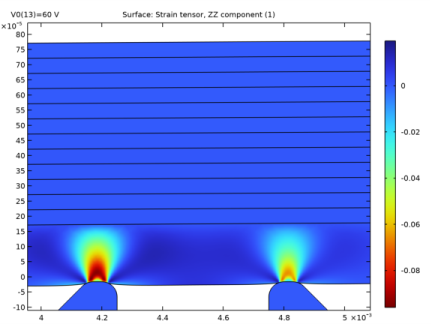
In the Settings window for Surface, click Replace Expression in the upper-right corner of the Expression section. From the menu, choose Component 1 (comp1)>Solid Mechanics>Strain>Strain tensor (material and geometry frames)>solid.eZZ - Strain tensor, ZZ component.
3
Locate the Coloring and Style section. From the Color table transformation list, choose Reverse.
4
In the Strain (ZZ component) toolbar, click  Plot.
Zoom in on the contact region and compare the plot with Figure 3.
Electric Field (Z component)
1
In the Model Builder window, right-click Strain (ZZ component) and choose Duplicate.
2
In the Model Builder window, click Strain (ZZ component) 1.
3
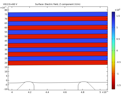
In the Settings window for 2D Plot Group, type Electric Field (Z component) in the Label text field.
Surface 1
1
In the Model Builder window, click Surface 1.
2
In the Settings window for Surface, click to collapse the Expression section.
3
Click Replace Expression in the upper-right corner of the Expression section. From the menu, choose Component 1 (comp1)>Electrostatics>Electric>Electric field (material and geometry frames) - V/m>es.EZ - Electric field, Z component.
4
In the Electric Field (Z component) toolbar, click  Plot.
Contact Pressure
1
In the Home toolbar, click  Add Plot Group and choose 1D Plot Group.
2
In the Settings window for 1D Plot Group, type Contact Pressure in the Label text field.
3
Locate the Data section. From the Parameter selection (V0) list, choose Last.
Line Graph 1
1
Right-click Contact Pressure and choose Line Graph.
2
3
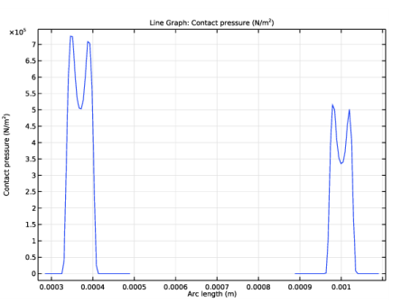
In the Settings window for Line Graph, click Replace Expression in the upper-right corner of the y-Axis Data section. From the menu, choose Component 1 (comp1)>Solid Mechanics>Contact>solid.Tn - Contact pressure - N/m².
4
In the Contact Pressure toolbar, click  Plot.
Appendix — Geometry Instructions
From the File menu, choose New.
New
In the New window, click  Model Wizard.
Model Wizard
1
In the Model Wizard window, click  2D Axisymmetric.
2
Global Definitions
Parameters 1
1
In the Model Builder window, under Global Definitions click Parameters 1.
2
In the Settings window for Parameters, locate the Parameters section.
3
Geometry 1
Rectangle 1 (r1)
1
In the Geometry toolbar, click  Rectangle.
2
In the Settings window for Rectangle, locate the Size and Shape section.
3
In the Width text field, type (OD-ID)/2.
4
In the Height text field, type t0.
5
Locate the Position section. In the r text field, type ID/2.
6
In the z text field, type ts.
7
Click to expand the Layers section. Select the Layers to the left check box.
8
Clear the Layers on bottom check box.
9
Array 1 (arr1)
1
In the Geometry toolbar, click  Transforms and choose Array.
2
In the Settings window for Array, locate the Size section.
3
In the z size text field, type n.
4
Locate the Displacement section. In the z text field, type t0.
5
Rectangle 2 (r2)
1
In the Geometry toolbar, click  Rectangle.
2
In the Settings window for Rectangle, locate the Size and Shape section.
3
In the Width text field, type 3*w0.
4
In the Height text field, type ts.
5
Locate the Position section. In the r text field, type ID/2+0.5*w0.
Fillet 1 (fil1)
1
In the Geometry toolbar, click  Fillet.
2
On the object r2, select Points 1 and 2 only.
3
In the Settings window for Fillet, locate the Radius section.
4
In the Radius text field, type ts/3.
Rectangle 3 (r3)
1
In the Geometry toolbar, click  Rectangle.
2
In the Settings window for Rectangle, locate the Size and Shape section.
3
In the Width text field, type 2*w0.
4
In the Height text field, type 2*w0+h0.
5
Locate the Position section. In the r text field, type ID/2-0.5*w0.
6
In the z text field, type -2*w0-deltaz-h0.
Chamfer 1 (cha1)
1
In the Geometry toolbar, click  Chamfer.
2
On the object r3, select Point 4 only.
3
In the Settings window for Chamfer, locate the Distance section.
4
In the Distance from vertex text field, type 1.8*w0.
Fillet 2 (fil2)
1
In the Geometry toolbar, click  Fillet.
2
On the object cha1, select Points 3 and 5 only.
3
In the Settings window for Fillet, locate the Radius section.
4
In the Radius text field, type 0.1*w0.
Polygon 1 (pol1)
1
In the Geometry toolbar, click  Polygon.
2
In the Settings window for Polygon, locate the Coordinates section.
3
Mirror 1 (mir1)
1
In the Geometry toolbar, click  Transforms and choose Mirror.
2
Select the objects fil2 and pol1 only.
3
In the Settings window for Mirror, locate the Input section.
4
Select the Keep input objects check box.
5
Locate the Point on Line of Reflection section. In the r text field, type ID/2+2*w0.
Rectangle 4 (r4)
1
In the Geometry toolbar, click  Rectangle.
2
In the Settings window for Rectangle, locate the Size and Shape section.
3
In the Width text field, type ID/2+1.5*w0.
4
In the Height text field, type h0.
5
Locate the Position section. In the z text field, type -2*w0-deltaz-h0.
Rectangle 5 (r5)
1
In the Geometry toolbar, click  Rectangle.
2
In the Settings window for Rectangle, locate the Size and Shape section.
3
In the Width text field, type OD/2+w1-ID/2-2.5*w0.
4
In the Height text field, type h0.
5
Locate the Position section. In the r text field, type ID/2+2.5*w0.
6
In the z text field, type -2*w0-deltaz-h0.
Rectangle 6 (r6)
1
In the Geometry toolbar, click  Rectangle.
2
In the Settings window for Rectangle, locate the Size and Shape section.
3
In the Width text field, type w2+w1.
4
In the Height text field, type h0+4*w0+n*t0+deltaz.
5
Locate the Position section. In the r text field, type OD/2-w2.
6
In the z text field, type -2*w0-deltaz-h0.
7
Click  Build Selected.