PDF

Pull-In Voltage for a Biased Resonator — 3D
Introduction
Silicon micromechanical resonators have long been used for designing sensors and are now becoming increasingly important as oscillators in the consumer electronics market. In this sequence of models, a surface micromachined MEMS resonator, designed as part of a micromechanical filter, is analyzed in detail. The resonator is based on that developed in Ref. 1.
This model performs a pull-in analysis of the structure, to predict the point at which the biased system becomes unstable. The analysis begins from the stationary analysis performed in the accompanying model Stationary Analysis of a Biased Resonator — 3D; please review this model first.
Model Definition
The geometry, fabrication, and operation of the device are discussed for the Stationary Analysis of a Biased Resonator — 3D model.
This model computes the pull-in voltage for the resonator by solving an inverse problem. The z-coordinate of the resonator midpoint is computed using an integration operator (intop1). The inverse problem that COMSOL solves computes the DC voltage that must be applied to the beam in order to move the midpoint to a set z-coordinate, zset. This is achieved by adding a global equation for the DC voltage, VdcSP, applied to the resonator. The equation intop1(z)-zset=0 is solved to determine the value of VdcSP. This means that VdcSP is adjusted until the midpoint of the resonator has a z-coordinate given by the set value, zset. Essentially COMSOL is being asked to find the voltage that allows the beam to exist in equilibrium (stable or unstable) at a given displacement. Solving the problem in this way avoids complications with trying to solve a problem with no solution (which is what happens if the voltage is continuously ramped up eventually exceeding the pull-in voltage). The result of the analysis is a displacement versus voltage plot, with a minimum at the pull-in voltage. Note that for a linear spring, the pull-in displacement corresponds to 1/3 of the gap distance. Although the inclusion of geometric nonlinearities in the solid mechanics solver means that the pull-in displacement changes slightly from this value, it is usually most efficient to search around this point for the pull-in voltage.
Results and Discussion
Figure 1 shows the voltage-displacement curve for the resonator at equilibrium. The y-coordinate at which the pull in occurs corresponds to a displacements around 1/3 of the gap size. The pull-in voltage is 59.1 V.
Figure 1: Voltage required to achieve a set displacement versus the target displacement. The pull-in voltage is the minimum of the plot: 59.4 V.
Figure 2: z-displacement of the resonator at pull-in. The displacement at pull-in is 75 nm. For a linear spring the displacement at pull in would be 66 nm.
Figure 2 shows the z-displacement of the resonator at the pull-in voltage. The maximum displacement at pull-in is 75 nm. This is comparable to the linear spring value of 66 nm.
Notes About the COMSOL Implementation
To compute the voltage required to generate the desired displacement of the beam, use a global equation. A common use of global equations is for computing the value of a dependent variable based on an ordinary differential equation in the dependent variable itself. However, it is also possible to couple a global equation with the other PDEs in the model as a powerful tool to solve certain kinds of inverse problems. This model uses a global equation to compute the potential applied to the drive electrode. The equation takes the form
where z0 is the z-coordinate of the midpoint of the beam’s underside and zset is the desired z-coordinate. COMSOL Multiphysics computes the voltage to satisfy the constraint implied by the above equation. Note that the large difference in scale between the set-point displacement (107 m) and the applied voltages (102 V) means that care must be taken with the dependent variable scaling in the solver settings.
Reference
1. F.D. Bannon III, J.R. Clark and C.T.-C. Nguyen, “High-Q HF Microelectromechanical Filters,” IEEE Journal of Solid State Circuits, vol. 35, no. 4, pp. 512–526, 2000.
Application Library path: MEMS_Module/Actuators/biased_resonator_3d_pull_in
Modeling Instructions
Open the existing stationary study (filename: biased_resonator_3d_basic.mph).
Application Libraries
1
From the File menu, choose Application Libraries.
2
In the Application Libraries window, select MEMS Module>Actuators>biased_resonator_3d_basic in the tree.
3
Add a parameter to set the z-coordinate of the midpoint of the resonator.
Global Definitions
Parameters 1
1
In the Model Builder window, under Global Definitions click Parameters 1.
2
In the Settings window for Parameters, locate the Parameters section.
3
Add a nonlocal integration coupling to compute the actual displacement.
Definitions
Integration 1 (intop1)
1
In the Model Builder window, expand the Component 1 (comp1) node.
2
Right-click Component 1 (comp1)>Definitions and choose Nonlocal Couplings>Integration.
3
In the Settings window for Integration, locate the Source Selection section.
4
From the Geometric entity level list, choose Point.
5
Change the drive potential to the value VdcSP - which will be solved for in a global equation.
Electrostatics (es)
Terminal 2
1
In the Model Builder window, expand the Component 1 (comp1)>Electrostatics (es) node, then click Terminal 2.
2
In the Settings window for Terminal, locate the Terminal section.
3
In the V0 text field, type VdcSP.
Add a global equation to compute the voltage for a given displacement, VdcSP.
4
Click the  Show More Options button in the Model Builder toolbar.
5
In the Show More Options dialog box, in the tree, select the check box for the node Physics>Equation-Based Contributions.
6
Global Equations 1
1
In the Physics toolbar, click  Global and choose Global Equations.
2
In the Settings window for Global Equations, locate the Global Equations section.
3
Set up a parametric sweep over zset.
Add Study
1
In the Home toolbar, click  Add Study to open the Add Study window.
2
Go to the Add Study window.
3
Find the Studies subsection. In the Select Study tree, select General Studies>Stationary.
4
Click Add Study in the window toolbar.
5
In the Home toolbar, click  Add Study to close the Add Study window.
Study 2
Step 1: Stationary
1
In the Settings window for Stationary, click to expand the Study Extensions section.
2
Select the Auxiliary sweep check box.
3
4
From the list in the Parameter name column, choose zset (Set point z-coordinate).
5
Click  Range.
6
In the Range dialog box, type 120e-9 in the Start text field.
7
In the Step text field, type 2e-9.
8
In the Stop text field, type 140e-9.
9
Click Replace.
The dependent variables require scaling correctly in order to assist the solver.
Solution 2 (sol2)
1
In the Study toolbar, click  Show Default Solver.
2
In the Model Builder window, expand the Solution 2 (sol2) node, then click Dependent Variables 1.
3
In the Settings window for Dependent Variables, locate the General section.
4
From the Defined by study step list, choose User defined.
5
In the Model Builder window, expand the Study 2>Solver Configurations>Solution 2 (sol2)>Dependent Variables 1 node, then click Electric potential (comp1.V).
6
In the Settings window for Field, locate the Scaling section.
7
From the Method list, choose Manual.
8
In the Scale text field, type 100.
9
In the Model Builder window, under Study 2>Solver Configurations>Solution 2 (sol2)>Dependent Variables 1 click Applied bias required to reach zset (V) (comp1.ODE1).
10
In the Settings window for State, locate the Scaling section.
11
From the Method list, choose Manual.
12
In the Scale text field, type 100.
The problem is highly nonlinear, so the solver settings need to be adjusted accordingly.
13
In the Model Builder window, expand the Study 2>Solver Configurations>Solution 2 (sol2)>Stationary Solver 1 node.
14
Right-click Study 2>Solver Configurations>Solution 2 (sol2)>Stationary Solver 1 and choose Fully Coupled.
15
In the Settings window for Fully Coupled, locate the General section.
16
From the Linear solver list, choose Direct.
17
Click to expand the Method and Termination section. From the Nonlinear method list, choose Automatic highly nonlinear (Newton).
18
In the Model Builder window, right-click Study 2 and choose Rename.
19
In the Rename Study dialog box, type Pull In in the New label text field.
20
Pull In
1
In the Model Builder window, click Pull In.
2
In the Study toolbar, click  Compute.
Results
Displacement (solid) 1
Determine the pull-in voltage by plotting VdcSP versus zset.
1D Plot Group 8
1
In the Home toolbar, click  Add Plot Group and choose 1D Plot Group.
2
In the Settings window for 1D Plot Group, locate the Data section.
3
From the Dataset list, choose Pull In/Solution 2 (sol2).
Global 1
1
Right-click 1D Plot Group 8 and choose Global.
2
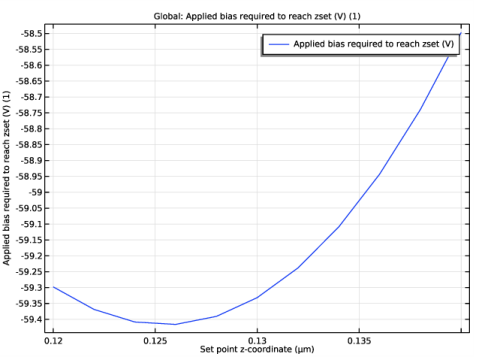
In the Settings window for Global, click Replace Expression in the upper-right corner of the y-Axis Data section. From the menu, choose Component 1 (comp1)>Electrostatics>VdcSP - Applied bias required to reach zset (V).
3
Locate the x-Axis Data section. From the Parameter list, choose Expression.
4
In the Expression text field, type zset.
Pull-In Plot
1
In the Model Builder window, right-click 1D Plot Group 8 and choose Rename.
2
In the Rename 1D Plot Group dialog box, type Pull-In Plot in the New label text field.
3
4
In the Pull-In Plot toolbar, click  Plot.
5
Click the  Zoom Extents button in the Graphics toolbar.
Compare the resulting plot with Figure 1. The pull in voltage is the minimum of the curve: 59.4 V at zset = 126 nm.
Now look at the displacement at pull in. The default plot group can be used.
Displacement (solid) 1
1
In the Model Builder window, click Displacement (solid) 1.
2
In the Settings window for 3D Plot Group, locate the Data section.
3
From the Parameter value (zset (m)) list, choose 1.24E-7.
4
In the Displacement (solid) 1 toolbar, click  Plot.
5
Click the  Zoom Extents button in the Graphics toolbar.
Compare the resulting plot with Figure 2. The displacement at pull-in is 75 nm.