|
|
|
|
•
|
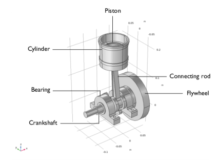
A Solid-Bearing Coupling multiphysics coupling is used to combine the engine-bearing assembly. The Hydrodynamic Journal Bearing in the Hydrodynamic Bearing physics interface is used to model the thin fluid film flow in the journal bearing. You need one such node per bearing.
|
|
•
|
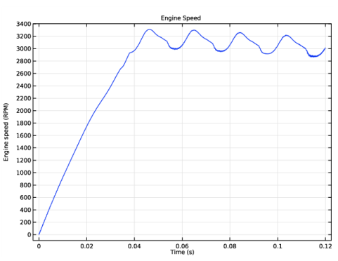
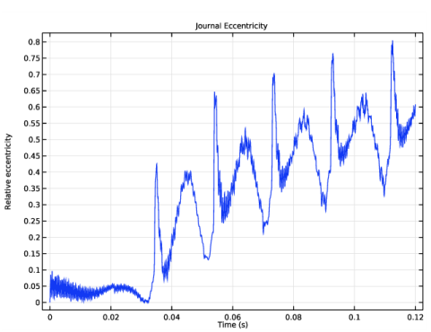
A hydrodynamic bearing can support the load only when the journal is running at a finite speed. In this model, the engine is started using an external torque on the crankshaft. Therefore, in the beginning the speed of the crankshaft is small and the bearings cannot support the load on the crankshaft from the connecting rod. A Hinge Joint with joint elasticity is used to support the crankshaft in the beginning. The elastic stiffness is slowly decreased to zero after the engine startup.
|
|
•
|
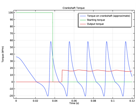
The Applied Moment subnode of the Rigid Connector is used to apply the starting and loading torque. Step functions are used to switch the two torques.
|
|
1
|
|
2
|
|
3
|
Click Add.
|
|
4
|
|
5
|
Click Add.
|
|
6
|
Click
|
|
7
|
|
8
|
Click
|
|
1
|
|
2
|
|
3
|
Click
|
|
4
|
Browse to the model’s Application Libraries folder and double-click the file single_cylinder_reciprocating_engine.mphbin.
|
|
5
|
Click
|
|
1
|
|
2
|
|
3
|
|
4
|
|
1
|
|
2
|
|
1
|
In the Model Builder window, under Component 1 (comp1)>Definitions, Ctrl-click to select Identity Boundary Pair 1 (ap1), Identity Boundary Pair 2 (ap2), Identity Boundary Pair 3 (ap3), and Identity Boundary Pair 5 (ap5).
|
|
2
|
Right-click and choose Group.
|
|
1
|
In the Model Builder window, under Component 1 (comp1)>Definitions click Identity Boundary Pair 4 (ap4).
|
|
2
|
|
3
|
|
1
|
In the Model Builder window, under Component 1 (comp1)>Definitions>Hinge Joint Pairs click Identity Boundary Pair 1 (ap1).
|
|
2
|
|
3
|
|
4
|
|
5
|
Click OK.
|
|
6
|
|
7
|
|
8
|
|
9
|
Click OK.
|
|
1
|
|
2
|
|
3
|
|
4
|
|
5
|
Click OK.
|
|
6
|
|
7
|
|
8
|
|
9
|
Click OK.
|
|
1
|
|
2
|
|
3
|
|
4
|
|
5
|
|
6
|
|
7
|
|
8
|
|
9
|
|
13
|
|
1
|
|
2
|
|
3
|
|
4
|
|
5
|
|
6
|
Click OK.
|
|
1
|
|
2
|
|
3
|
|
4
|
|
5
|
|
6
|
|
7
|
|
8
|
Click OK.
|
|
1
|
|
2
|
|
3
|
|
4
|
|
5
|
|
6
|
|
7
|
|
8
|
Click OK.
|
|
1
|
|
2
|
|
3
|
|
4
|
|
5
|
|
6
|
|
7
|
|
1
|
|
2
|
|
3
|
|
1
|
|
2
|
|
3
|
|
1
|
|
2
|
|
3
|
|
1
|
|
2
|
|
3
|
|
4
|
|
5
|
In the Add dialog box, in the Selections to add list, choose Fixed 1, Fixed 2, Fixed 3, and Fixed 4.
|
|
6
|
Click OK.
|
|
1
|
|
2
|
|
3
|
|
4
|
|
5
|
|
6
|
|
1
|
|
2
|
|
3
|
|
4
|
|
5
|
|
1
|
|
2
|
|
3
|
|
4
|
|
5
|
|
6
|
|
1
|
|
2
|
|
3
|
|
4
|
|
5
|
|
6
|
Browse to the model’s Application Libraries folder and double-click the file single_cylinder_reciprocating_engine_pressure_data.txt.
|
|
7
|
|
8
|
In the Function table, enter the following settings:
|
|
1
|
|
2
|
|
3
|
|
4
|
|
5
|
|
1
|
In the Model Builder window, under Component 1 (comp1) right-click Multibody Dynamics (mbd) and choose Material Models>Rigid Domain.
|
|
2
|
In the Settings window for Rigid Domain, in the Graphics window toolbar, click
|
|
4
|
|
1
|
|
3
|
|
1
|
|
3
|
|
4
|
|
5
|
|
6
|
|
7
|
|
8
|
Click Physics Node Generation in the upper-right corner of the Automated Model Setup section. From the menu, choose Create Joints.
|
|
1
|
|
2
|
|
1
|
In the Model Builder window, under Component 1 (comp1)>Multibody Dynamics (mbd)>Hinge Joints click Attachment 2.
|
|
2
|
|
1
|
|
2
|
|
3
|
|
1
|
|
2
|
|
3
|
|
1
|
In the Model Builder window, under Component 1 (comp1)>Multibody Dynamics (mbd)>Hinge Joints click Attachment 3.
|
|
2
|
|
1
|
In the Model Builder window, under Component 1 (comp1)>Multibody Dynamics (mbd)>Hinge Joints click Attachment 4.
|
|
2
|
|
1
|
In the Model Builder window, under Component 1 (comp1)>Multibody Dynamics (mbd)>Hinge Joints click Attachment 5.
|
|
2
|
|
1
|
|
2
|
|
3
|
|
1
|
|
2
|
|
3
|
|
1
|
|
2
|
|
3
|
|
4
|
Click Physics Node Generation in the upper-right corner of the Automated Model Setup section. From the menu, choose Create Joints.
|
|
1
|
|
2
|
|
3
|
|
1
|
In the Model Builder window, under Component 1 (comp1) right-click Definitions and choose Variables.
|
|
2
|
|
1
|
|
2
|
|
3
|
|
4
|
|
5
|
|
1
|
|
2
|
In the Settings window for Rigid Connector, in the Graphics window toolbar, click
|
|
1
|
|
2
|
|
3
|
Specify the M vector as
|
|
1
|
|
2
|
|
3
|
Specify the M vector as
|
|
4
|
|
5
|
|
6
|
|
1
|
|
2
|
|
3
|
|
4
|
|
5
|
In the Show More Options dialog box, in the tree, select the check box for the node Physics>Advanced Physics Options.
|
|
6
|
Click OK.
|
|
7
|
|
8
|
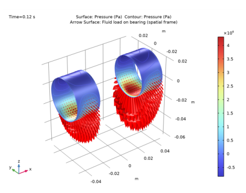
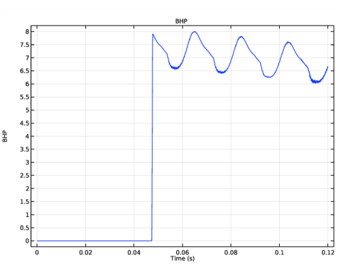
Select the Cavitation check box.
|
|
1
|
In the Model Builder window, under Component 1 (comp1)>Hydrodynamic Bearing (hdb) click Hydrodynamic Journal Bearing 1.
|
|
2
|
|
3
|
|
4
|
Locate the Fluid Properties section. From the μ list, choose User defined. In the associated text field, type mu0.
|
|
5
|
|
1
|
Right-click Component 1 (comp1)>Hydrodynamic Bearing (hdb)>Hydrodynamic Journal Bearing 1 and choose Duplicate.
|
|
2
|
|
3
|
|
1
|
|
2
|
|
3
|
|
4
|
|
5
|
|
1
|
|
2
|
|
3
|
|
4
|
|
1
|
|
2
|
|
3
|
|
4
|
|
5
|
Click OK.
|
|
1
|
|
2
|
|
3
|
|
5
|
|
6
|
|
1
|
|
2
|
|
3
|
|
4
|
|
5
|
In the Add dialog box, in the Selections to add list, choose Bearing Exterior Edges and Foundation Exterior Edges.
|
|
6
|
Click OK.
|
|
7
|
|
1
|
|
2
|
|
3
|
|
1
|
|
3
|
In the Settings window for Distribution, in the Graphics window toolbar, click
|
|
5
|
|
1
|
|
2
|
|
3
|
|
4
|
|
1
|
|
2
|
|
3
|
|
4
|
|
1
|
|
2
|
|
3
|
|
1
|
|
2
|
|
3
|
|
4
|
|
1
|
|
2
|
|
3
|
|
1
|
|
2
|
|
3
|
|
4
|
|
5
|
In the Model Builder window, expand the Study 1>Solver Configurations>Solution 1 (sol1)>Time-Dependent Solver 1 node, then click Fully Coupled 1.
|
|
6
|
|
7
|
|
8
|
|
9
|
|
10
|
|
1
|
|
2
|
|
3
|
|
1
|
|
2
|
In the Settings window for Selection, in the Graphics window toolbar, click
|
|
3
|
|
1
|
In the Model Builder window, under Results>Datasets right-click Study 1/Solution 1: Cylinder (sol1) and choose Duplicate.
|
|
2
|
|
3
|
In the Settings window for Solution, type Study 1/Solution 1: Engine without cylinder in the Label text field.
|
|
1
|
|
2
|
|
3
|
|
1
|
|
2
|
|
3
|
|
1
|
|
2
|
|
3
|
|
4
|
|
5
|
|
6
|
|
1
|
|
2
|
|
3
|
|
1
|
|
2
|
|
1
|
|
2
|
|
3
|
|
4
|
|
5
|
|
1
|
In the Model Builder window, under Results>Datasets right-click Study 1/Solution 1 (sol1) and choose Duplicate.
|
|
2
|
|
1
|
|
2
|
|
3
|
|
4
|
|
1
|
|
2
|
|
3
|
|
4
|
|
5
|
|
1
|
|
2
|
|
3
|
|
4
|
|
5
|
|
6
|
|
7
|
|
8
|
|
9
|
|
10
|
|
1
|
In the Model Builder window, under Results>Datasets right-click Study 1/Solution 1 (sol1) and choose Duplicate.
|
|
2
|
|
1
|
|
2
|
|
3
|
|
1
|
In the Model Builder window, under Results>Datasets right-click Study 1/Solution 1: Crankshaft (sol1) and choose Duplicate.
|
|
2
|
|
1
|
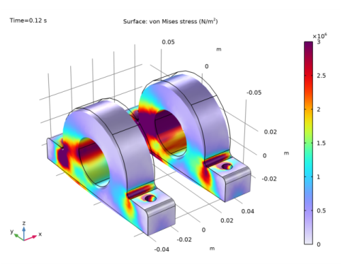
In the Model Builder window, expand the Results>Datasets>Study 1/Solution 1: Foundation (sol1) node, then click Selection.
|
|
2
|
|
3
|
|
4
|
|
1
|
|
2
|
|
3
|
|
1
|
|
2
|
|
3
|
|
4
|
|
5
|
|
6
|
|
1
|
|
2
|
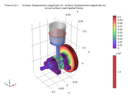
In the Settings window for Deformation, click Replace Expression in the upper-right corner of the Expression section. From the menu, choose Component 1 (comp1)>Multibody Dynamics>Displacement>u_ref,...,w_ref - Displacement field, reference frame (spatial frame).
|
|
3
|
Locate the Scale section.
|
|
4
|
|
1
|
|
2
|
|
3
|
|
4
|
|
5
|
|
6
|
|
1
|
|
2
|
|
3
|
|
4
|
|
5
|
|
6
|
|
7
|
|
1
|
|
2
|
|
3
|
|
1
|
|
2
|
In the Settings window for Deformation, click Replace Expression in the upper-right corner of the Expression section. From the menu, choose Component 1 (comp1)>Multibody Dynamics>Displacement>u,v,w - Displacement field.
|
|
3
|
|
1
|
|
2
|
|
1
|
|
2
|
|
1
|
|
2
|
|
4
|
|
1
|
|
2
|
|
3
|
|
4
|
|
5
|
|
6
|
|
1
|
|
2
|
In the Settings window for 1D Plot Group, type Bearing Reactions and Piston Load in the Label text field.
|
|
1
|
|
2
|
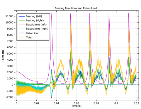
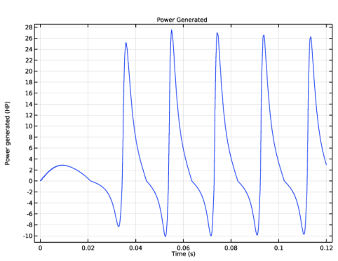
In the Settings window for Global, click Replace Expression in the upper-right corner of the y-Axis Data section. From the menu, choose Component 1 (comp1)>Hydrodynamic Bearing>Fluid loads>Fluid load on journal (spatial frame) - N>hdb.hjb1.Fjz - Fluid load on journal, z component.
|
|
3
|
Click Add Expression in the upper-right corner of the y-Axis Data section. From the menu, choose Component 1 (comp1)>Hydrodynamic Bearing>Fluid loads>Fluid load on journal (spatial frame) - N>hdb.hjb2.Fjz - Fluid load on journal, z component.
|
|
4
|
Click Add Expression in the upper-right corner of the y-Axis Data section. From the menu, choose Component 1 (comp1)>Multibody Dynamics>Hinge joints>Hinge Joint 1>Joint force (elastic) - N>mbd.hgj1.F_elz - Joint force (elastic), z component.
|
|
5
|
Click Add Expression in the upper-right corner of the y-Axis Data section. From the menu, choose Component 1 (comp1)>Multibody Dynamics>Hinge joints>Hinge Joint 3>Joint force (elastic) - N>mbd.hgj3.F_elz - Joint force (elastic), z component.
|
|
6
|
|
7
|
|
1
|
|
2
|
|
3
|
|
4
|
|
5
|
|
6
|
|
7
|
|
1
|
|
2
|
|
3
|
|
4
|
|
5
|
|
1
|
|
2
|
|
4
|
|
1
|
|
2
|
|
1
|
|
2
|
|
4
|
|
5
|
|
1
|
|
2
|
|
3
|
|
4
|
|
1
|
|
2
|
|
3
|
|
1
|
|
2
|
|
4
|
|
1
|
|
2
|
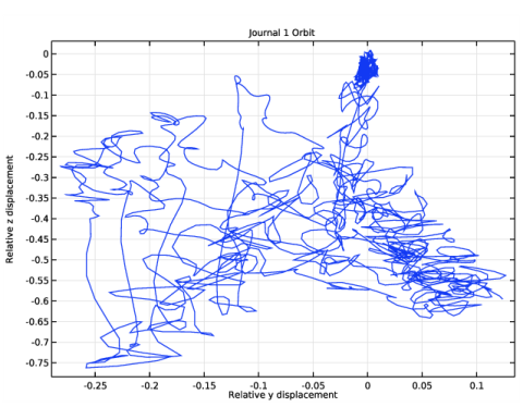
In the Settings window for Global, click Replace Expression in the upper-right corner of the y-Axis Data section. From the menu, choose Component 1 (comp1)>Multibody Dynamics>Attachments>Attachment: Journal 1>Rigid body displacement (spatial frame) - m>mbd.att1.w - Rigid body displacement, z component.
|
|
3
|
|
4
|
|
5
|
Click Replace Expression in the upper-right corner of the x-Axis Data section. From the menu, choose Component 1 (comp1)>Multibody Dynamics>Attachments>Attachment: Journal 1>Rigid body displacement (spatial frame) - m>mbd.att1.v - Rigid body displacement, y component.
|
|
6
|
|
7
|
|
1
|
|
2
|
|
3
|
|
4
|
|
5
|
|
6
|
|
7
|
|
8
|
|
1
|
|
2
|
|
3
|
|
4
|
|
1
|
|
2
|
|
4
|
|
5
|
|
1
|
|
2
|
|
3
|
|
4
|
|
5
|
|
6
|
|
7
|
|
1
|
|
2
|
|
3
|
|
4
|
|
5
|
|
6
|
|
7
|
|
8
|
|
1
|
|
2
|
|
3
|
|
4
|
|
5
|
|
6
|
|
7
|