|
|
|
|
•
|
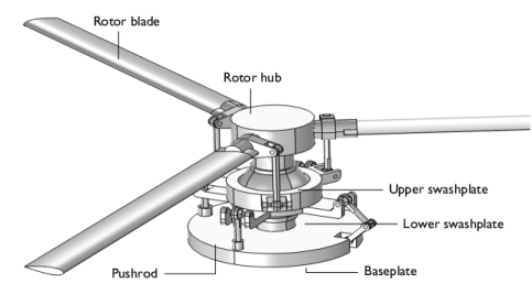
Pushrod (3 in number, stationary)
|
|
•
|
Baseplate-Swashplate Link (2 in number, stationary)
|
|
•
|
Rotor Blade (3 in number, rotating)
|
|
•
|
Swashplate-Blade Link (3 in number, rotating)
|

|
•
|
|
•
|
Cl — lift coefficient
|
|
•
|
Ur — relative velocity at a point over the rotor blades
|
|
•
|
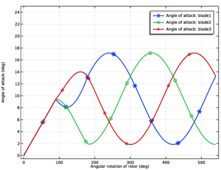
α — angle of attack of rotor blades
|
|
•
|
ω — angular velocity of rotor blades
|
|
•
|
vf — forward speed of helicopter
|
|
•
|
d — distance of a point over the rotor blades from the center of rotation
|
|
•
|
x, y — spatial coordinates of a point over the rotor blades
|
|
•
|
A Joint node can establish a direct connection between Rigid Domain nodes. However, for flexible elements, Attachment nodes are needed to define the connection boundaries.
|
|
•
|
Constraint boundary conditions like Rigid Connector and Prescribed Displacement cannot be used with a Rigid Domain node. Hence, the Prescribed Displacement/Rotation node (subnode to Rigid Domain) is used to constrain or prescribe the corresponding degrees of freedom.
|
|
•
|
The connections set up in the model can be reviewed in the Joints Summary section at the physics node.
|
|
1
|
|
2
|
|
3
|
Click Add.
|
|
4
|
Click
|
|
5
|
|
6
|
Click
|
|
1
|
|
2
|
|
3
|
Click
|
|
4
|
Browse to the model’s Application Libraries folder and double-click the file helicopter_swashplate.mphbin.
|
|
5
|
Click
|
|
6
|
|
1
|
|
2
|
|
3
|
Select the Cutoff check box.
|
|
5
|
|
6
|
|
7
|
|
8
|
|
1
|
|
2
|
|
3
|
|
4
|
|
5
|
|
1
|
|
2
|
|
1
|
|
2
|
|
1
|
|
2
|
|
1
|
|
2
|
|
1
|
|
2
|
|
3
|
|
4
|
|
5
|
Click OK.
|
|
1
|
|
2
|
|
3
|
|
4
|
|
5
|
Click OK.
|
|
1
|
|
2
|
|
3
|
|
4
|
|
5
|
|
1
|
|
2
|
|
3
|
Specify the ω vector as
|
|
1
|
|
2
|
|
4
|
|
1
|
|
2
|
|
4
|
|
1
|
|
2
|
|
1
|
|
2
|
|
3
|
|
4
|
Locate the Prescribed Displacement at Center of Rotation section. Select the Prescribed in x direction check box.
|
|
5
|
|
6
|
|
7
|
|
8
|
Specify the Ω vector as
|
|
9
|
|
1
|
|
2
|
In the Settings window for Rigid Domain, type Rigid Domain: Upper Swashplate in the Label text field.
|
|
1
|
|
2
|
|
1
|
|
2
|
|
3
|
|
4
|
|
5
|
|
6
|
|
1
|
In the Model Builder window, expand the Prismatic Joint 1 node, then click Center of Joint: Point 1.
|
|
1
|
|
2
|
|
3
|
|
1
|
|
2
|
|
3
|
|
4
|
|
5
|
|
6
|
Locate the Axes of Joint section. From the Joint translational axis list, choose Attached on source.
|
|
7
|
|
8
|
|
1
|
In the Model Builder window, expand the Reduced Slot Joint 1 node, then click Center of Joint: Point 1.
|
|
1
|
|
2
|
|
3
|
|
4
|
Locate the Prescribed Rotational Motion section. From the Activation condition list, choose Never active.
|
|
1
|
|
2
|
|
3
|
|
4
|
|
5
|
|
6
|
|
1
|
In the Model Builder window, expand the Prismatic Joint 2 node, then click Center of Joint: Point 1.
|
|
1
|
|
2
|
|
3
|
|
1
|
|
2
|
|
3
|
|
4
|
|
5
|
|
1
|
|
1
|
|
1
|
|
2
|
|
3
|
|
4
|
|
5
|
|
1
|
|
1
|
|
1
|
|
2
|
|
3
|
|
4
|
|
5
|
|
1
|
|
1
|
|
2
|
|
3
|
|
4
|
|
5
|
|
6
|
|
1
|
|
2
|
|
3
|
|
4
|
|
5
|
|
6
|
|
1
|
|
2
|
|
3
|
|
1
|
|
2
|
|
3
|
|
4
|
|
5
|
|
1
|
|
1
|
|
2
|
|
3
|
|
4
|
|
5
|
Locate the Variables section. In the table, enter the following settings:
|
|
1
|
|
2
|
|
3
|
|
4
|
|
5
|
Locate the Variables section. In the table, enter the following settings:
|
|
1
|
|
2
|
|
3
|
|
4
|
|
5
|
Locate the Variables section. In the table, enter the following settings:
|
|
1
|
|
2
|
|
3
|
|
5
|
|
1
|
|
2
|
|
3
|
|
1
|
|
2
|
|
3
|
|
1
|
|
2
|
|
3
|
|
1
|
|
2
|
|
1
|
|
3
|
|
4
|
|
1
|
|
2
|
|
3
|
|
4
|
|
5
|
|
1
|
|
2
|
|
3
|
In the Model Builder window, under Study: Rigid Blades>Solver Configurations>Solution 1 (sol1) click Time-Dependent Solver 1.
|
|
4
|
|
5
|
|
6
|
|
1
|
|
2
|
|
3
|
|
1
|
|
2
|
|
3
|
|
4
|
|
5
|
|
1
|
|
2
|
|
3
|
Locate the Physics and Variables Selection section. Select the Modify model configuration for study step check box.
|
|
4
|
In the tree, select Component 1 (Comp1)>Multibody Dynamics (Mbd)>Rigid Domain: Rotor Blade1, Component 1 (Comp1)>Multibody Dynamics (Mbd)>Rigid Domain: Rotor Blade2, and Component 1 (Comp1)>Multibody Dynamics (Mbd)>Rigid Domain: Rotor Blade3.
|
|
5
|
Right-click and choose Disable.
|
|
6
|
|
7
|
|
8
|
|
9
|
|
1
|
|
2
|
|
3
|
|
4
|
|
1
|
|
2
|
|
1
|
|
2
|
|
3
|
|
4
|
|
5
|
|
1
|
In the Model Builder window, expand the Study: Flexible Blades/Solution 2 (4) (sol2) node, then click Selection.
|
|
2
|
|
3
|
|
4
|
|
5
|
|
1
|
|
2
|
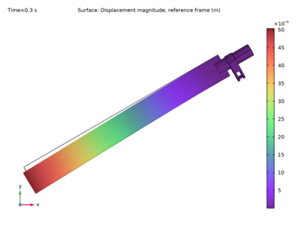
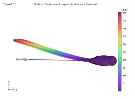
In the Settings window for 3D Plot Group, type Displacement: Flexible Blade1 in the Label text field.
|
|
3
|
Locate the Data section. From the Dataset list, choose Study: Flexible Blades/Solution 2 (3) (sol2).
|
|
4
|
|
5
|
|
6
|
|
1
|
|
2
|
|
3
|
|
1
|
|
2
|
|
3
|
|
4
|
|
5
|
|
6
|
|
1
|
|
2
|
|
3
|
|
4
|
|
5
|
|
6
|
|
7
|
|
8
|
|
9
|
|
10
|
|
11
|
|
1
|
|
2
|
|
3
|
Locate the Data section. From the Dataset list, choose Study: Flexible Blades/Solution 2 (2) (sol2).
|
|
4
|
|
5
|
|
1
|
|
2
|
|
3
|
|
4
|
|
5
|
|
6
|
|
7
|
|
8
|
|
1
|
|
2
|
|
3
|
|
4
|
|
5
|
|
6
|
|
1
|
|
2
|
|
3
|
|
4
|
|
5
|
|
6
|
|
7
|
|
1
|
|
2
|
|
3
|
|
4
|
|
5
|
|
6
|
|
1
|
|
2
|
|
1
|
|
2
|
|
4
|
|
5
|
|
6
|
|
7
|
|
8
|
|
1
|
|
2
|
|
3
|
|
4
|
In the associated text field, type Angular rotation of rotor (deg).
|
|
5
|
|
6
|
In the associated text field, type Angle of attack (deg).
|
|
7
|
|
8
|
|
9
|
|
10
|
|
11
|
|
1
|
|
2
|
|
3
|
|
4
|
|
1
|
|
2
|
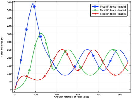
In the Settings window for Global, click Replace Expression in the upper-right corner of the y-Axis Data section. From the menu, choose Component 1 (comp1)>Definitions>Variables>FL_tot1 - Total lift force - blade1 - N.
|
|
3
|
Click Add Expression in the upper-right corner of the y-Axis Data section. From the menu, choose Component 1 (comp1)>Definitions>Variables>FL_tot2 - Total lift force - blade2 - N.
|
|
4
|
Click Add Expression in the upper-right corner of the y-Axis Data section. From the menu, choose Component 1 (comp1)>Definitions>Variables>FL_tot3 - Total lift force - blade3 - N.
|
|
5
|
|
6
|
|
7
|
|
8
|
|
1
|
|
2
|
|
3
|
|
4
|
In the associated text field, type Angular rotation of rotor (deg).
|
|
5
|
|
6
|
In the associated text field, type Total lift force (N).
|
|
7
|
|
8
|
|
1
|
|
2
|
|
3
|
|
1
|
|
2
|
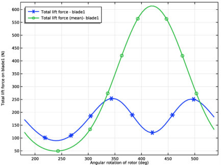
In the Settings window for Global, click Replace Expression in the upper-right corner of the y-Axis Data section. From the menu, choose Component 1 (comp1)>Definitions>Variables>FL_tot1 - Total lift force - blade1 - N.
|
|
3
|
Click Add Expression in the upper-right corner of the y-Axis Data section. From the menu, choose Component 1 (comp1)>Definitions>Variables>FL_tot1_alphaM - Total lift force (mean)- blade1 - N.
|
|
1
|
|
2
|
|
3
|
|
4
|
|
5
|
|
6
|
|
1
|
|
2
|
|
1
|
|
2
|
|
3
|
|
4
|
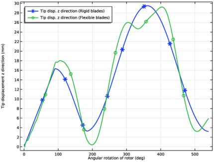
Click Replace Expression in the upper-right corner of the y-Axis Data section. From the menu, choose Component 1 (comp1)>Definitions>Variables>w_tip - Tip displacement z direction - m.
|
|
5
|
|
6
|
|
7
|
|
8
|
|
9
|
|
10
|
|
1
|
|
2
|
|
3
|
|
4
|
Locate the Legends section. In the table, enter the following settings:
|
|
1
|
|
2
|
|
3
|
|
4
|
|
5
|
|
6
|
In the associated text field, type Angular rotation of rotor (deg).
|
|
7
|
|
1
|
|
2
|
|
3
|
|
4
|
|
5
|
|
1
|
|
2
|
|
4
|
Locate the Physics and Variables Selection section. Select the Modify model configuration for study step check box.
|
|
5
|
In the tree, select Component 1 (Comp1)>Multibody Dynamics (Mbd)>Rigid Domain: Rotor Blade1, Component 1 (Comp1)>Multibody Dynamics (Mbd)>Rigid Domain: Rotor Blade2, Component 1 (Comp1)>Multibody Dynamics (Mbd)>Rigid Domain: Rotor Blade3, Component 1 (Comp1)>Multibody Dynamics (Mbd)>Prismatic Joint 1>Prescribed Motion 1, Component 1 (Comp1)>Multibody Dynamics (Mbd)>Reduced Slot Joint 1>Prescribed Motion 1, and Component 1 (Comp1)>Multibody Dynamics (Mbd)>Prismatic Joint 2>Prescribed Motion 1.
|
|
6
|
Right-click and choose Disable.
|
|
7
|
|
8
|
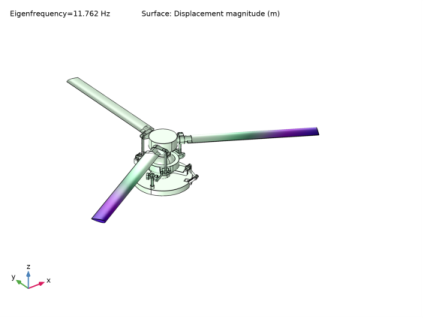
In the Settings window for Study, type Study: Flexible Blades[Eigenfrequency] in the Label text field.
|
|
9
|
|
1
|
|
2
|
|
3
|
|
4
|
|
1
|
In the Model Builder window, expand the Results>Mode Shape (mbd)>Surface node, then click Deformation.
|
|
2
|
|
3
|
|
1
|
|
2
|
|
3
|
|
4
|
|
5
|
|
1
|
|
2
|
|
3
|
|
1
|
|
2
|
|
3
|
|
1
|
|
2
|
|
3
|