|
|
|
|
•
|
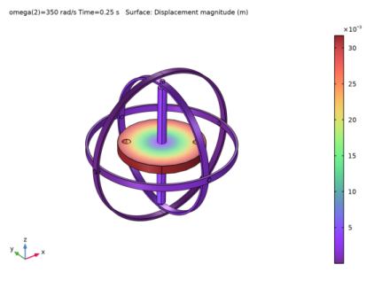
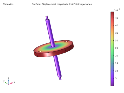
In this model, parts are modeled as rigid elements using the Rigid Domain node as we are only interested in the kinematics of the mechanism. Parts can be modeled as flexible elements using the Linear Elastic Material node if the stresses and deformations in the parts are also of interest.
|

|
1
|
|
2
|
|
3
|
Click Add.
|
|
4
|
Click
|
|
5
|
|
6
|
Click
|
|
1
|
|
2
|
|
1
|
|
2
|
|
1
|
|
2
|
|
3
|
Click
|
|
4
|
|
5
|
Click
|
|
1
|
In the Model Builder window, under Component 1: Gyroscope (comp1)>Geometry 1 click Form Union (fin).
|
|
2
|
|
3
|
|
4
|
|
5
|
|
1
|
|
2
|
|
3
|
|
4
|
|
1
|
|
2
|
|
3
|
In the tree, select Built-in>Aluminum.
|
|
4
|
|
5
|
|
6
|
|
7
|
|
1
|
In the Model Builder window, under Component 1: Gyroscope (comp1) right-click Multibody Dynamics (mbd) and choose Material Models>Rigid Domain.
|
|
2
|
|
1
|
|
2
|
In the Settings window for Prescribed Displacement/Rotation, locate the Prescribed Displacement at Center of Rotation section.
|
|
3
|
|
4
|
|
5
|
|
6
|
|
7
|
Specify the Ω vector as
|
|
8
|
|
1
|
|
2
|
|
1
|
|
2
|
|
1
|
|
2
|
|
4
|
|
1
|
|
2
|
|
3
|
Specify the ω vector as
|
|
1
|
|
2
|
|
3
|
|
4
|
|
5
|
|
1
|
|
2
|
|
3
|
|
4
|
|
5
|
|
1
|
|
2
|
|
3
|
|
4
|
|
5
|
|
1
|
|
2
|
|
3
|
|
4
|
|
1
|
In the Model Builder window, under Component 1: Gyroscope (comp1) right-click Definitions and choose Variables.
|
|
2
|
|
1
|
|
2
|
|
3
|
|
1
|
|
2
|
|
1
|
|
2
|
|
3
|
Click
|
|
1
|
|
2
|
|
3
|
|
1
|
|
2
|
|
3
|
|
4
|
|
5
|
|
6
|
|
1
|
|
2
|
|
3
|
|
4
|
|
5
|
|
6
|
|
1
|
|
2
|
|
3
|
|
4
|
|
5
|
|
1
|
|
2
|
|
3
|
|
4
|
|
5
|
|
6
|
|
1
|
|
2
|
|
3
|
Locate the Data section. From the Dataset list, choose Study 1: Gyroscope/Parametric Solutions 1 (sol2).
|
|
4
|
|
5
|
|
1
|
|
2
|
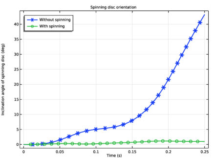
In the Settings window for Global, click Replace Expression in the upper-right corner of the y-Axis Data section. From the menu, choose Component 1: Gyroscope (comp1)>Definitions>Variables>theta - Inclination angle of spinning disc - rad.
|
|
3
|
|
4
|
|
5
|
|
6
|
|
7
|
|
9
|
|
10
|
|
1
|
|
2
|
|
3
|
Click
|
|
4
|
|
5
|
Click
|
|
1
|
|
2
|
|
3
|
|
4
|
On the object imp1(1), select Domain 1 only.
|
|
5
|
On the object imp1(2), select Domain 1 only.
|
|
6
|
|
7
|
|
1
|
|
2
|
Select the object imp1(3) only.
|
|
3
|
|
4
|
|
5
|
|
6
|
|
7
|
|
1
|
|
2
|
|
3
|
|
1
|
|
2
|
|
3
|
In the tree, select Built-in>Aluminum.
|
|
4
|
|
5
|
|
1
|
|
2
|
|
3
|
|
4
|
Find the Physics interfaces in study subsection. In the table, clear the Solve check box for Study 1: Gyroscope.
|
|
5
|
|
6
|
|
1
|
Right-click Component 2: Spinning top (comp2)>Multibody Dynamics 2 (mbd2) and choose Material Models>Rigid Domain.
|
|
3
|
|
4
|
|
1
|
|
2
|
|
3
|
|
4
|
|
5
|
|
6
|
|
1
|
|
1
|
|
2
|
In the Settings window for Prescribed Displacement/Rotation, locate the Prescribed Displacement at Center of Rotation section.
|
|
3
|
|
4
|
|
5
|
|
6
|
|
7
|
|
1
|
|
1
|
|
1
|
In the Model Builder window, under Component 2: Spinning top (comp2) right-click Definitions and choose Variables.
|
|
2
|
|
1
|
|
2
|
|
3
|
|
1
|
|
2
|
|
3
|
|
4
|
Find the Physics interfaces in study subsection. In the table, clear the Solve check box for Multibody Dynamics (mbd).
|
|
5
|
|
6
|
|
7
|
|
1
|
|
2
|
|
3
|
|
1
|
|
2
|
|
3
|
|
4
|
|
5
|
|
6
|
|
1
|
|
3
|
|
4
|
|
1
|
|
2
|
|
3
|
|
4
|
|
5
|
|
1
|
|
2
|
|
3
|
|
4
|
|
5
|
|
6
|
|
7
|
|
8
|
|
1
|
|
2
|
|
3
|
|
4
|
|
5
|
|
6
|
|
1
|
|
2
|
|
3
|
|
4
|
|
5
|
|
6
|
|
7
|
|
8
|
|
1
|
|
3
|
|
4
|
|
5
|
|
6
|
|
7
|
|
8
|
|
9
|
|
1
|
|
2
|
|
3
|
|
4
|
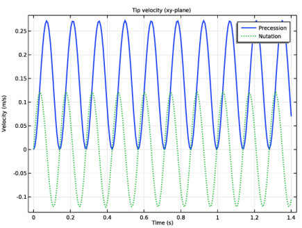
In the associated text field, type Velocity (m/s).
|
|
5
|
|
6
|
|
1
|
|
2
|
In the Settings window for Point Graph, click Replace Expression in the upper-right corner of the y-Axis Data section. From the menu, choose Component 2: Spinning top (comp2)>Definitions>Variables>vp - Precession velocity - m/s.
|
|
3
|
|
4
|
Locate the Coloring and Style section. Find the Line style subsection. From the Line list, choose Cycle.
|
|
5
|
|
6
|
|
1
|
|
2
|
In the Settings window for Point Graph, click Replace Expression in the upper-right corner of the y-Axis Data section. From the menu, choose Component 2: Spinning top (comp2)>Definitions>Variables>vn - Nutation velocity - m/s.
|
|
3
|
Locate the Legends section. In the table, enter the following settings:
|
|
4
|
|
5
|