PDF

Modeling Vibration and Noise in a Gearbox: CMS Version
Introduction
A gearbox is used for transferring power from the engine to the wheels. Predicting the vibration and noise radiation from a dynamic system like a gearbox gives designers an insight early in the design process.
When operated, a gearbox can radiate noise in the surrounding because of two reasons. The first and foremost one is the transmission of undesired lateral and axial forces on the bearings and housing while transmitting power from one shaft to another. The second reason is the flexibility in the different parts of the gearbox such as the gear mesh, bearings, and housing.
This example illustrates the modeling of vibration and noise in a 5-speed synchromesh gearbox of a manual transmission vehicle. A transient multibody analysis is performed to compute the gearbox vibration for the specified engine speed and external load. The normal acceleration of the gearbox housing is converted to the frequency domain and used as a source of noise. An acoustics analysis is then performed in order to compute the sound pressure levels in the near, far, and exterior fields.
This example is essentially the same as Modeling Vibration and Noise in a Gearbox, but with the flexible gearbox housing reduced to a computationally efficient reduced-order model (ROM) using the Component Mode Synthesis (CMS) technique.
Model Definition
Figure 1: The modeled geometry of a 5-speed synchromesh gearbox of a manual transmission vehicle.
The geometry of a synchromesh gearbox is shown in Figure 1. Only those parts of the gearbox which are relevant from a physics point of view are considered for the analysis.
The gearbox has a varying gear mesh stiffness which causes vibrations. These vibrations are transmitted to the gearbox housing, and the vibrating housing further transmits the energy to the surrounding fluid, resulting in radiation of acoustic waves. In order to study this phenomena numerically, the following analyses are performed:
Additional information regarding the gear arrangements, loads, constraints, connections, boundary conditions for multibody and acoustics analyses can be found in the documentation for Modeling Vibration and Noise in a Gearbox.
This example focuses on the reduction of the flexible housing using the CMS technique, the details of which are discussed in the following.
Component mode synthesis (CMS)
The CMS technique reduces flexible components to computationally efficient ROMs using a number of constraint modes and eigenmodes for each individual component.
In COMSOL, the CMS technique is implemented within the Reduced Flexible Components node of the Multibody Dynamics interface. The steps needed to set up a CMS model are described below.
Component Definition
In the Reduced Flexible Components node, all flexible components which are supposed to be reduced can be selected together. By default, individual components are detected automatically using the geometric connectivity information. In this example, there is only one flexible component, the gearbox housing.
Note: The Reduced Flexible Components node allows only elastic domains and it is not possible to, for example, select rigid domains. Hence, in this model, it is possible to select all domains of the geometry, and automatically only elastic domains will be applicable.
Connection Boundaries
The next step is to define a set of connection boundaries on each component using Attachment nodes. In a typical multibody dynamics model, such nodes are present in the model. Otherwise, it is possible to add more Attachment nodes as needed.
Constraint Modes
The number of constraint modes for each component is automatically computed using the number of connection boundaries, that is, the number of attachments. For this 3D example, each attachment sets up six constraint modes: three translations and three rotations. Given that the housing has four attachments, a total of 24 constraint modes are computed.
Eigenmodes
A number of eigenmodes are required for the reduction of dynamic problems. This is a user input, and the number of eigenmodes has a direct effect on the accuracy and performance, hence, it has to be chosen wisely. Ideally, the eigenmodes used to approximate the solution should cover the frequency range of the particular dynamic problem. For this example, the first 50 eigenmodes are considered.
Configure CMS Study
The next step is to configure a CMS study with Parametric Sweep, Stationary, Eigenfrequency, and Model Reduction study steps. This is done by clicking the Configure CMS Study button in the Reduced Flexible Components node. If changes are made in the model after configuring the study, it is advisable to reconfigure the CMS study.
Generating Reduced Components
When computing the CMS study, ROMs corresponding to each flexible component are generated. These appear as Reduced Component nodes under the Reduced-Order Modeling node in the Global Definitions branch.
Using Reduced Components
The next step is to use these generated reduced components in any existing or new study. These reduced components are, by default, linked to the Reduced Flexible Components node and are automatically solved, or not solved, based on whether this node is enabled or disabled in a particular study step. Hence, in general, there is no extra step needed in order to use reduced components.
Field Reconstruction
While working with reduced components, the states of the ROMs are dependent variables. Since these are global degrees of freedom, a reconstruction of the displacement field is required in order to evaluate or plot any field variable. This is done by default within the Reduced Flexible Components node, which makes it possible to plot or evaluate any field variable in postprocessing, including stresses and strains. Also, such reconstructed field variables can seamlessly be used for any multiphysics coupling, for example, transferring the normal acceleration of the elastic housing to the acoustics analysis in order to predict the generation of noise.
Results and Discussion
The multibody dynamics analysis of the gearbox is performed in the time domain for one revolution of the main shaft. The von Mises stress distribution in the housing at a particular instant is shown in Figure 2. The speed of different gears can also be seen in the figure.
Figure 2: Distribution of von Mises stress in the housing at t = 0.0754 s. The speed of different gears is also shown.
While the gearbox is in operation, it starts vibrating under the influence of various forces. The normal acceleration of the housing, a measure of the noise radiation, is shown in Figure 3 for a particular instance in time. In order to understand its variation in time, Figure 4 show the time history for a point at the top of the gearbox. In this figure, the normal acceleration is plotted as a function of the main shaft rotation.
In order to get a better understanding about the frequency content, we can transform these results to the frequency domain by using the FFT solver; the results of this operation are shown in Figure 5. It is clear from the plot that the normal acceleration of the housing definitely contains more than one frequency. The frequency band in which the housing vibration is dominant is 1000 Hz to 3000 Hz.
The sound pressure level in the near field as well as on the surface of the gearbox housing is shown in Figure 6 and Figure 7, respectively. The sound pressure level at the far field in different planes can be seen in Figure 8, Figure 9, and Figure 10. These far-fields plots of the sound pressure level give a clear idea about the directivity of noise radiation at a particular frequency.
Figure 3: Normal acceleration of the housing at t = 0.0754 s. The speed of the different gears is also shown.
Figure 4: Time history of the normal acceleration at one of the points at the top of the gearbox.
Figure 5: Frequency spectrum of the normal acceleration at one of the points at the top of the gearbox.
Figure 6: Sound pressure level outside the gearbox at 2000 Hz.
Figure 7: Sound pressure level at the surface of the gearbox at 2000 Hz.
Figure 8: Far-field sound pressure level at a distance of 1 m in the xy-plane at 2000 Hz.
Figure 9: Far-field sound pressure level at a distance of 1 m in the xz-plane at 2000 Hz.
Figure 10: Far-field sound pressure level at a distance of 1 m in the yz-plane at 2000 Hz.
The pressure magnitude at two microphone locations as a function of frequency is shown in Figure 11. It can be seen that the magnitude of the pressure at microphone 1 is higher than the second one, since it is nearer to the source of noise.
In order to visualize the pressure wave propagation in the air domain outside the gearbox, the frequency domain pressure data can be converted back to the time domain. The pressure field at a particular instance in time is shown in Figure 12.
Figure 11: Frequency spectrum of the pressure magnitude at two microphone locations.
Figure 12: Total acoustics pressure field outside the gearbox at  t= 0.00377 s.
Notes About the COMSOL Implementation
Application Library path: Multibody_Dynamics_Module/Automotive_and_Aerospace/gearbox_vibration_noise_cms
Modeling Instructions
Root
In this example you will start from an existing model from the Multibody Dynamics Module.
Application Libraries
1
From the File menu, choose Application Libraries.
2
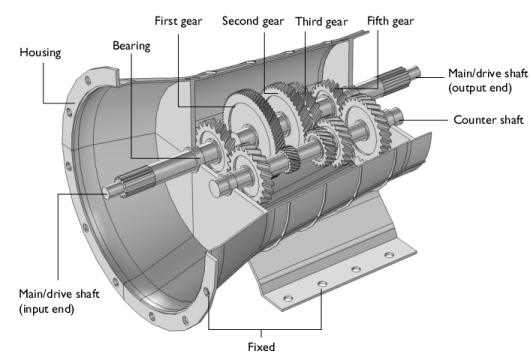
In the Application Libraries window, select Multibody Dynamics Module>Automotive and Aerospace>gearbox_vibration_noise in the tree.
3
Component 1 (comp1)
Add a Reduced Flexible Components node to reduce the flexible casing of the gearbox using the CMS technique.
1
In the Model Builder window, expand the Component 1 (comp1) node.
Multibody Dynamics (mbd)
Reduced Flexible Components 1
1
In the Model Builder window, expand the Component 1 (comp1)>Multibody Dynamics (mbd) node.
2
Right-click Multibody Dynamics (mbd) and choose More>Reduced Flexible Components.
3
In the Settings window for Reduced Flexible Components, locate the Domain Selection section.
4
From the Selection list, choose All domains.
To accurately capture high-frequency vibrations, use at least the first 50 eigenmodes of the flexible casing. Subsequently generate a CMS study node to compute the reduced-order model of the casing.
5
Locate the Component Mode Synthesis section. In the Number of eigenmodes text field, type 50.
6
Click CMS Configuration in the upper-right corner of the Component Mode Synthesis section. From the menu, choose Configure CMS Study.
CMS Study
1
In the Home toolbar, click  Compute.
The reduced-order model of the casing is generated by the CMS study node. It is available under the Global Definitions node. The next step is to use this reduced-order model in the time-dependent study.
Study: Multibody Analysis
Solution 1 (sol1)
1
In the Model Builder window, expand the Study: Multibody Analysis node.
2
Right-click Solver Configurations and choose Reset Solver to Default.
3
In the Model Builder window, expand the Solution 1 (sol1) node, then click Time-Dependent Solver 1.
4
In the Settings window for Time-Dependent Solver, click to expand the Time Stepping section.
5
From the Steps taken by solver list, choose Intermediate.
6
In the Home toolbar, click  Compute.
Various plots are already available in the model. Browse through these default plots to analyze the results.
Results
Velocity - Stress
1
In the Velocity - Stress toolbar, click  Plot.
2
Click the  Zoom Extents button in the Graphics toolbar.
Velocity - Normal Acceleration
1
In the Model Builder window, click Velocity - Normal Acceleration.
2
In the Velocity - Normal Acceleration toolbar, click  Plot.
3
Click the  Zoom Extents button in the Graphics toolbar.
Normal Acceleration
1
In the Model Builder window, click Normal Acceleration.
2
In the Normal Acceleration toolbar, click  Plot.
3
Click the  Zoom Extents button in the Graphics toolbar.
Normal Acceleration: Frequency
1
In the Model Builder window, click Normal Acceleration: Frequency.
2
In the Normal Acceleration: Frequency toolbar, click  Plot.
3
Click the  Zoom Extents button in the Graphics toolbar.
Now run the acoustics analysis in the model to compute the noise radiation from the gearbox.
Component 2 (comp2)
In the Model Builder window, expand the Component 2 (comp2) node.
Pressure Acoustics, Frequency Domain (acpr)
Normal Acceleration 1
1
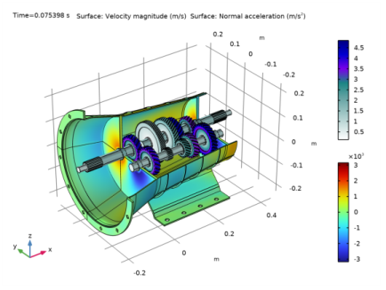
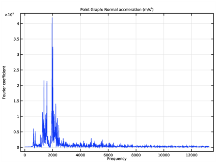
In the Model Builder window, expand the Component 2 (comp2)>Pressure Acoustics, Frequency Domain (acpr) node, then click Normal Acceleration 1.
2
In the Settings window for Normal Acceleration, locate the Normal Acceleration section.
3
Specify the a0 vector as
Study: Acoustics (Frequency Domain)
In the Home toolbar, click  Compute.
Again, browse through the default plots to analyze the results.
Results
SPL Near Field
1
In the SPL Near Field toolbar, click  Plot.
2
Click the  Zoom Extents button in the Graphics toolbar.
SPL Casing Surface
1
In the Model Builder window, click SPL Casing Surface.
2
In the SPL Casing Surface toolbar, click  Plot.
3
Click the  Zoom Extents button in the Graphics toolbar.
Polar SPL xy-plane
1
In the Model Builder window, click Polar SPL xy-plane.
2
In the Polar SPL xy-plane toolbar, click  Plot.
3
Click the  Zoom Extents button in the Graphics toolbar.
Polar SPL xz-plane
1
In the Model Builder window, click Polar SPL xz-plane.
2
In the Polar SPL xz-plane toolbar, click  Plot.
3
Click the  Zoom Extents button in the Graphics toolbar.
Polar SPL yz-plane
1
In the Model Builder window, click Polar SPL yz-plane.
2
In the Polar SPL yz-plane toolbar, click  Plot.
3
Click the  Zoom Extents button in the Graphics toolbar.
Microphone Pressure
1
In the Model Builder window, click Microphone Pressure.
2
In the Microphone Pressure toolbar, click  Plot.
3
Click the  Zoom Extents button in the Graphics toolbar.
Study: Acoustics (Time Domain)
In the Home toolbar, click  Compute.
Results
Pressure Near Field: Time
1
In the Pressure Near Field: Time toolbar, click  Plot.
2
Click the  Zoom Extents button in the Graphics toolbar.