|
|
|
|
tr, tp
|
|
•
|
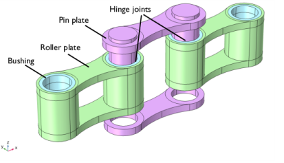
Pin Outer Boundaries: This is a boundary selection containing the outer cylindrical surfaces of all the pin plates. The selection is used for creating Attachment nodes for each of the pin plates.
|
|
•
|
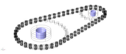
Roller Inner Boundaries: This is a boundary selection containing inner cylindrical surfaces of all the roller plates. This selection is used for creating Attachment nodes for each of the roller plates. The selection coincides geometrically with the Pin Outer Boundaries (Figure 3). The attachments for the pin and roller plates are used as Source and Destination in Hinge Joint nodes.
 |
|
•
|
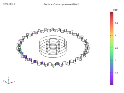
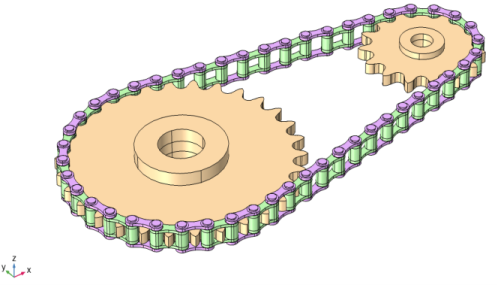
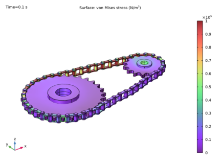
Roller Outer Boundaries: This boundary selection contains the outer cylindrical surfaces of all the roller plates. The selection is used for creating Contact Pair nodes for modeling contact between links and sprockets, as shown in Figure 4.
|
|
•
|
Sprocket Outer Boundaries: This boundary selection contains the outer surfaces of the sprockets. The selection is used for creating a Contact Pair for modeling contact between links and sprockets as shown in Figure 4.
 |
|
•
|
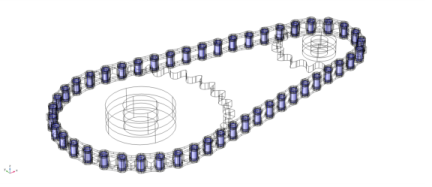
Sprocket Inner Boundaries: This boundary selection contains the inner surfaces of the sprockets, as shown in Figure 5. It is used for creating attachments and hinge joints for mounting the sprockets onto shafts.
 |
|
•
|
To build a chain drive system geometry, you can import a roller chain sprocket assembly part from the Part Library, and customize it by changing its input parameters.
|
|
•
|
The Chain Drive node operates on the geometry in the assembly state.
|
|
•
|
The Chain Drive node creates new physics nodes from selections available in the geometry. If you are using a part imported from the Part Library, select the check box in Geometry to keep noncontributing selections. If you are building a geometry of a roller chain and sprocket assembly, you also need to create appropriate selections for the Chain Drive node to operate.
|
|
•
|
When one or more selection inputs of the Chain Drive node change, the selections of the physics nodes created by Chain Drive node also change. Hence, these nodes have to be deleted and recreated. This is indicated by a warning node appearing under the Chain Drive node. In that case, you need to press the Create Links and Joints button. This will automatically create new groups of physics nodes in accordance with the changed selection inputs.
|
|
1
|
|
2
|
|
3
|
Click Add.
|
|
4
|
Click
|
|
5
|
|
6
|
Click
|
|
1
|
|
2
|
|
1
|
|
2
|
|
3
|
|
4
|
|
1
|
|
2
|
|
3
|
|
1
|
|
2
|
In the Part Libraries window, select Multibody Dynamics Module>3D>Roller Chains>roller_chain_sprocket_assembly in the tree.
|
|
3
|
|
4
|
In the Select Part Variant dialog box, select Specify sprocket center distance in the Select part variant list.
|
|
5
|
Click OK.
|
|
1
|
In the Model Builder window, under Component 1 (comp1)>Geometry 1 click Roller Chain Sprocket 1 (pi1).
|
|
2
|
|
3
|
|
4
|
|
1
|
|
2
|
|
3
|
|
4
|
|
5
|
|
1
|
|
2
|
|
3
|
|
4
|
|
5
|
|
1
|
In the Model Builder window, under Component 1 (comp1) right-click Multibody Dynamics (mbd) and choose Chain Drive.
|
|
2
|
|
3
|
|
4
|
|
5
|
|
1
|
|
2
|
|
3
|
|
4
|
|
1
|
|
2
|
|
3
|
From the list, choose Joint.
|
|
4
|
|
1
|
In the Model Builder window, expand the Component 1 (comp1)>Multibody Dynamics (mbd)>cdr1: Contact node, then click Contact: Sprocket-Roller (cdr1).
|
|
2
|
|
3
|
|
4
|
|
1
|
In the Model Builder window, under Component 1 (comp1) right-click Definitions and choose Variables.
|
|
2
|
|
1
|
|
2
|
|
1
|
|
2
|
|
1
|
|
2
|
|
3
|
|
4
|
|
1
|
|
2
|
|
3
|
|
1
|
|
2
|
|
3
|
|
4
|
|
5
|
In the Model Builder window, expand the Study 1>Solver Configurations>Solution 1 (sol1)>Time-Dependent Solver 1 node, then click Fully Coupled 1.
|
|
6
|
|
7
|
|
8
|
|
1
|
|
2
|
|
1
|
|
2
|
|
3
|
|
4
|
|
5
|
|
6
|
|
1
|
|
2
|
|
3
|
|
4
|
|
5
|
|
6
|
|
1
|
|
2
|
|
3
|
|
1
|
|
2
|
|
3
|
|
4
|
|
5
|
|
6
|
|
7
|
|
8
|
|
1
|
|
2
|
|
3
|
|
5
|
|
6
|
|
1
|
|
2
|
|
3
|
|
5
|
|
6
|
|
1
|
|
2
|
|
3
|
|
4
|
|
5
|
|
6
|
Click
|
|
1
|
|
2
|
In the Settings window for 3D Plot Group, type Contact Pressure, Sprocket-1 in the Label text field.
|
|
3
|
|
4
|
|
5
|
Locate the Selection section. From the Selection list, choose First Sprocket (Roller Chain Sprocket 1).
|
|
6
|
|
7
|
|
1
|
|
2
|
|
3
|
|
1
|
|
2
|
|
3
|
|
4
|
|
5
|
|
1
|
|
2
|
|
3
|
|
4
|
|
5
|
|
6
|
In the associated text field, type Force (N).
|
|
7
|
|
1
|
|
2
|
|
4
|
|
1
|
|
2
|
|
3
|
|
1
|
|
2
|
|
3
|
|
1
|
|
2
|
|
3
|
|
1
|
|
2
|
|
3
|
|
1
|
|
2
|
|
3
|