PDF

Magnetic Brake — LiveLink™ for Simulink® Simulation
Introduction
A magnet brake in its simplest form consists of a disc of conductive material and a permanent magnet, as in Figure 1 below, represented in orange and light gray, respectively. The magnet generates a constant magnetic field, in which the disc is rotating. When a conductor moves in a magnetic field it induces currents, and the Lorentz forces from the currents slow the disc. This model is variant of the Magnetic Brake model from the AC/DC Module Application Library, where the angular velocity is computed in Simulink based on the induced torque and the disk moment of inertia.
Figure 1: Conceptual geometry of a magnet brake.
Note: This models requires licenses for both the AC/DC Module and LiveLink™ for Simulink®.
Model Definition
The relation between the induced torque Tz and the angular velocity ω can be described by an ordinary differential equation (ODE):
Here, I is the moment of inertia of the disk.
The induced torque is computed in COMSOL Multiphysics as a 3D electromagnetic stationary problem.
The cosimulation with COMSOL Multiphysics and Simulink is set up by exporting a COMSOL Cosimulation file from the COMSOL model and then adding this to the COMSOL Cosimulation block in the Simulink simulation diagram. The input of the block consists of the angular velocity ω, provided by Simulink using an integrator block. The block output is the ratio .
Figure 2 shows the full simulation diagram in Simulink.
Figure 2: The simulation control diagram.
The initial velocity of the disc is 1000 rpm. To see the effect of the remanent flux in the magnet, a second input is set to the COMSOL block; the focus in this simulation is a constant value of 1 T.
Results and Discussion
Figure 3 below shows the current density in the disk at initial rotating velocity (1000 rpm).
Figure 3: Norm of the current density in the disk at maximal rotating velocity.
 Figure 4 shows the decrease of rotational velocity with a 1 T remanent flux density norm.
Figure 4: Angular velocity versus time.
Setting Up the Cosimulation
Follow the workflow below to set up the cosimulation with COMSOL Multiphysics and Simulink:
1
2
3
4
5
6
Application Library path: LiveLink_for_Simulink/Tutorials/magnetic_brake_llsimulink
Modeling Instructions — COMSOL Desktop
In this example you will start from an existing model which is an example described in the AC/DC Module Application Libraries.
Application Libraries
1
From the File menu, choose Application Libraries.
2
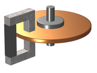
In the Application Libraries window, select ACDC Module>Motors and Actuators>magnetic_brake in the tree.
3
Global Definitions
Parameters 1
1
In the Model Builder window, under Global Definitions click Parameters 1.
2
In the Settings window for Parameters, locate the Parameters section.
3
Component 1 (comp1)
In the Model Builder window, expand the Component 1 (comp1) node.
Magnetic and Electric Fields (mef)
Velocity (Lorentz Term) 2
1
In the Model Builder window, expand the Component 1 (comp1)>Magnetic and Electric Fields (mef) node.
2
Right-click Component 1 (comp1)>Magnetic and Electric Fields (mef)>Velocity (Lorentz Term) 1 and choose Duplicate.
3
In the Settings window for Velocity (Lorentz Term), locate the Velocity (Lorentz Term) section.
4
Specify the v vector as
5
Right-click Velocity (Lorentz Term) 2 and choose Move Up.
Add Study
1
In the Home toolbar, click  Add Study to open the Add Study window.
2
Go to the Add Study window.
3
Find the Studies subsection. In the Select Study tree, select General Studies>Stationary.
4
5
In the Home toolbar, click  Add Study to close the Add Study window.
Study 2
Step 1: Stationary
1
In the Settings window for Stationary, locate the Physics and Variables Selection section.
2
Select the Modify model configuration for study step check box.
3
In the tree, select Component 1 (Comp1)>Magnetic and Electric Fields (Mef)>Velocity (Lorentz Term) 1.
4
5
In the tree, select Component 1 (Comp1)>Global ODEs and DAEs (Ge).
6
Click  Disable in Model.
7
In the Model Builder window, click Study 2.
8
In the Settings window for Study, locate the Study Settings section.
9
Clear the Generate default plots check box.
10
In the Home toolbar, click  Compute.
Results
3D Plot Group 5
1
In the Model Builder window, under Results right-click 3D Plot Group 4 and choose Duplicate.
2
In the Settings window for 3D Plot Group, locate the Data section.
3
From the Dataset list, choose Study 2/Solution 3 (sol3).
4
In the 3D Plot Group 5 toolbar, click  Plot.
Save the COMSOL Model
1
From the File menu, choose Save As.
2
Browse to a suitable folder, enter the filename magnetic_brake_llsimulink.mph, and then click Save.
Exporting the Cosimulation File
In the following configure the cosimulation, and export the file for cosimulation that will be loaded into Simulink.
Global Definitions
Cosimulation for Simulink 1
1
In the Study toolbar, click  Cosimulation for Simulink.
2
In the Settings window for Cosimulation for Simulink, locate the Filename section.
3
In the Filename text field, type magnetic_brake_llsimulink.
4
Locate the Inputs section. Click  Add.
5
6
Click to expand the Block Parameters section. Click  Add.
7
8
Locate the Outputs section. In the table, enter the following settings:
9
Locate the Image section. Click  Set from Graphics WindowThis sets the current temperature plot (if a solution is available) as the thumbnail used for the COMSOL Cosimulation block inside Simulink.
10
Click  Export.
Modeling Instructions — Simulink
Once you have created the COMSOL model and saved the cosimulation file you can start Simulink to continue with the setup there.
1
2
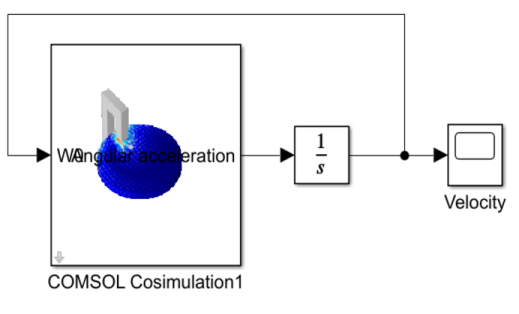
In MATLAB enter the command mphapplicationlibraries to start the GUI for viewing models from the LiveLink for Simulink application library.
3
4
The included COMSOL Cosimulation block is already configured with a cosimulation file based on the model from the COMSOL Application Library and ready to run. If you want to run the simulation directly, go to Step 7 below. Else, if you want to use the model file and cosimulation file you have created by following the steps in the section Modeling Instructions — COMSOL Desktop, you can continue with Step 5 below.
5
6
Note: In case the folder path of the file for cosimulation for Simulink is not set in MATLAB enter the full filename.
7
The simulation instruction are now over, you can run again a simulation with different settings such as the remanent flux in the magnet or the initial velocity.
If you want to change the remanent flux double-click the COMSOL Cosimulation block, then click Block parameters button. In the mB edit field, enter the desired value in Tesla and click OK.
If you want to change the initial velocity, double-click the Integrator block. In the Intial condition edit field enter the desired initial velocity in radian per seconds.