PDF

Homogenization in a Chemical Reactor
Introduction
This example illustrates how to simulate a periodic homogenization process in a space dependent chemical reactor model. This homogenization removes concentration gradients in the reactor at a set time interval.
The example demonstrates a technique by which you can implement the stopping of the time-dependent solver, then restarting it with an initial value obtained based on the solution.
Model Definition
The example studies the concentration of a diluted species in a reactor. The chemical reaction is defined by the reaction rate kc. Only the diffusion transport is considered in the example, no convection term is included.
The initial species concentration in the reactor is 0 and a fixed concentration of 1 mol/m3 is applied at the bottom boundary.
The homogenization takes place every 30 minutes, and it is assumed to be ideal. Thus, a homogeneous concentration is calculated as the average concentration in the reactor each time the solution is stopped. This concentration is then applied as the initial condition each time the solution is restarted.
Results and Discussion
Figure 1 shows the distribution of the concentration in the reactor after 30 minutes. The highest concentration appears close to the source boundary, while the lowest concentration is in the corner furthest away from it.
Figure 1: Concentration distribution after 30 minutes.
Figure 2 shows the concentration at the center of the top surface, defined by the coordinates (0.25m; 0.25m; 0.25m). The solid line denotes the concentration with the homogenization process. The dashed red line denotes the concentration when solving without homogenizing.
Figure 2: Evolution of the species concentration at (0.25m, 0.25m, 0.25m)
After 30 minutes the concentration in this point is much lower than the average value in the reactor. This can be seen by the jump in the concentration as the solver is restarted.
As evident from the figure the steady-state value for the concentration can be reached faster when applying the homogenization steps.
Notes About the COMSOL Implementation
The most efficient approach for this simulation is to start by setting up the diffusion problem in the graphical user interface of the COMSOL Desktop®. You can then save the model .mph file, which you can easily load into MATLAB®, where you continue to implement the script for solving the problem, including the homogenization steps.
Wrapper functions used by the script:
mphopen to load the model .mph file.
mphmean to evaluate the average concentration in the reactor.
mphinterp to evaluate the concentration at specific locations.
mphglobal to evaluate global quantities in the model.
mphplot to display plots.
Application Library path: LiveLink_for_MATLAB/Tutorials/homogenization_llmatlab
Modeling Instructions — MATLAB®
In this section you find a detailed explanation of the commands you need to enter at the MATLAB command line in order to run the simulation.
1
Start COMSOL with MATLAB.
You now have two possibilities to continue:
Enter each command, starting at step 2 below, at the MATLAB command line.
Paste the full model script, included in the section Model M-File, into a text editor, then save the file with a “.m” extension, and finally run this file in MATLAB.
2
model = mphopen('homogenization_llmatlab');
Note: See the section Modeling Instructions — COMSOL Desktop for the modeling instruction of the model .mph file homogenization_llmatlab.mph.
3
for i = 1:5
4
model.study('std1').run;
For the first iteration of the for loop the solver will stop after 30 minutes, according to the parameters, t0 and T, specified in the model. For each subsequent iteration the solution will run for an additional 30 minutes, as you are changing the value of the start time t0 in steps 7 and 8 below.
5
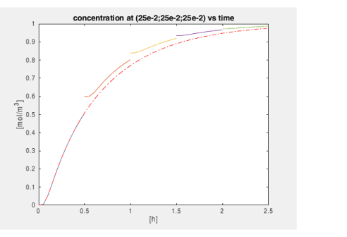
To obtain data for the plot shown in Figure 2 extract the concentration value at the specified location. Use the function mphinterp as shown below:
[t,c] = mphinterp(model,{'t','c'},...
   'coord',[25e-2;25e-2;25e-2],...
   'unit',{'h','mol/m^3'});
Now you can calculate the homogenized average concentration, which is the total amount of the substance, by integrating the concentration over the volume, and divide it by the reactor volume.
6
c_av = mphmean(model,'c','volume','solnum','end');
7
t0 = mphglobal(model,'t','solnum','end');
With the MATLAB variables c_av and t0 define a new initial concentration and start time for the next re-start of the solver, in the next iteration of the for-loop.
8
model.physics('tds').feature('init1').set('initc', 1, c_av);
model.param.set('t0',t0);
9
plot(t,c)
hold on
disp(sprintf('End of iteration No.%d',i));
10
end
11
title('concentration at (25e-2;25e-2;25e-2) vs time')
xlabel('[h]');
ylabel('[mol/m^3]');
12
model.param.set('t0',0);
model.param.set('tf','2.5[h]');
model.physics('tds').feature('init1').set('initc', 1, 0);
13
model.study('std1').run;
14
[t,c] = mphinterp(model,{'t','c'},...
   'coord',[25e-2;25e-2;25e-2],...
   'unit',{'h','mol/m^3'});
plot(t,c,'r-.')
15
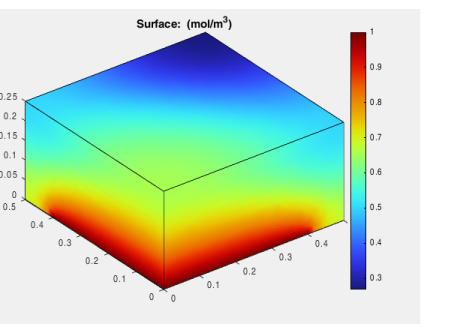
To reproduce the plot in Figure 1, you can also define a plot group in the model:
model.result.create('pg1', 'PlotGroup3D');
model.result('pg1').feature.create('surf1', 'Surface');
model.result('pg1').set('solnum', '11');
16
figure
mphplot(model,'pg1','rangenum',1)
Model M-File
Below you find the full script of the model. You can copy it and paste it into a text editor and save it with the “.m” extension. To run the script in MATLAB make sure that the path to the folder containing the script is set in MATLAB, then type the file name without the “.m” extension at the MATLAB prompt.
model = mphopen('homogenization_llmatlab');
 
for i = 1:5
   model.study('std1').run;
   [t,c] = mphinterp(model,{'t','c'},...
      'coord',[25e-2;25e-2;25e-2],...
      'unit',{'h','mol/m^3'});
   c_av = mphmean(model,'c','volume','solnum','end');
   t0 = mphglobal(model,'t','solnum','end');
   model.physics('tds').feature('init1').set('initc', 1, c_av);
   model.param.set('t0',t0);
   plot(t,c)
   hold on
   disp(sprintf('End of iteration No.%d',i));
end
 
title('concentration at (25e-2;25e-2;25e-2) vs time')
xlabel('[h]');
ylabel('[mol/m^3]')
 
model.param.set('t0',0);
model.param.set('tf','2.5[h]');
model.physics('tds').feature('init1').set('initc', 1, 0);
model.study('std1').run;
 
[t,c] = mphinterp(model,{'t','c'},...
   'coord',[25e-2;25e-2;25e-2],...
   'unit',{'h','mol/m^3'});
plot(t,c,'r-.')
 
model.result.create('pg1', 'PlotGroup3D');
model.result('pg1').feature.create('surf1', 'Surface');
model.result('pg1').set('solnum', '11');
 
figure
mphplot(model,'pg1','rangenum',1)
Modeling Instructions — COMSOL Desktop
Use the COMSOL Desktop to set-up the simulation of the chemical reactor. You can later load this example into MATLAB, using LiveLink™, to continue the model implementation.
From the File menu, choose New.
New
In the New window, click  Model Wizard.
Model Wizard
1
In the Model Wizard window, click  3D.
2
In the Select Physics tree, select Chemical Species Transport>Transport of Diluted Species (tds).
3
Click Add.
4
Click  Study.
5
In the Select Study tree, select General Studies>Time Dependent.
6
Global Definitions
Parameters 1
1
In the Model Builder window, under Global Definitions click Parameters 1.
2
In the Settings window for Parameters, locate the Parameters section.
3
Geometry 1
Block 1 (blk1)
1
In the Geometry toolbar, click  Block.
2
In the Settings window for Block, locate the Size and Shape section.
3
In the Width text field, type L.
4
In the Depth text field, type L.
5
In the Height text field, type L/2.
Work Plane 1 (wp1)
1
In the Geometry toolbar, click  Work Plane.
2
In the Settings window for Work Plane, click  Show Work Plane.
Work Plane 1 (wp1)>Plane Geometry
In the Model Builder window, click Plane Geometry.
Work Plane 1 (wp1)>Circular Arc 1 (ca1)
1
In the Work Plane toolbar, click  More Primitives and choose Circular Arc.
2
In the Settings window for Circular Arc, locate the Properties section.
3
From the Specify list, choose Endpoints and start angle.
4
Locate the Starting Point section. In the xw text field, type 4/5*L.
5
Locate the Endpoint section. In the yw text field, type 4/5*L.
6
Locate the Angles section. In the Start angle text field, type 0.
Form Union (fin)
In the Model Builder window, under Component 1 (comp1)>Geometry 1 right-click Form Union (fin) and choose Build Selected.
Transport of Diluted Species (tds)
Transport Properties 1
1
In the Model Builder window, under Component 1 (comp1)>Transport of Diluted Species (tds) click Transport Properties 1.
2
In the Settings window for Transport Properties, locate the Diffusion section.
3
In the Dc text field, type D.
Reactions 1
1
In the Physics toolbar, click  Domains and choose Reactions.
2
3
In the Settings window for Reactions, locate the Reaction Rates section.
4
In the Rc text field, type k*c.
Concentration 1
1
In the Physics toolbar, click  Boundaries and choose Concentration.
2
3
In the Settings window for Concentration, locate the Concentration section.
4
Select the Species c check box.
5
In the c0,c text field, type c0.
Mesh 1
Free Tetrahedral 1
In the Mesh toolbar, click  Free Tetrahedral.
Size 1
1
Right-click Free Tetrahedral 1 and choose Size.
2
In the Settings window for Size, locate the Geometric Entity Selection section.
3
From the Geometric entity level list, choose Boundary.
4
5
Locate the Element Size section. From the Predefined list, choose Extra fine.
6
Click  Build All.
Study 1
Step 1: Time Dependent
1
In the Model Builder window, under Study 1 click Step 1: Time Dependent.
2
In the Settings window for Time Dependent, locate the Study Settings section.
3
In the Output times text field, type range(t0,dt,tf).
Save the Model
1
2
Browse to a directory which path is set in MATLAB and enter domain_activation_llmatlab in the File name text field.
3
Click Save.