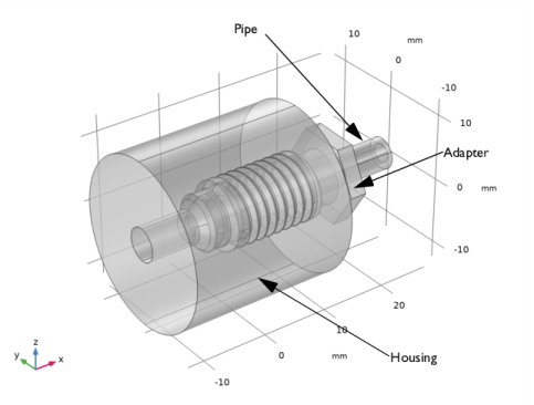
You are viewing the documentation for an older COMSOL version. The latest version is available here.
PDF

Stress Analysis of a Pipe Fitting from a CAD File
Introduction
The stress analysis of a threaded connection is usually a complex undertaking because of the presence of fine geometrical details. One way to simplify the problem is to assume that the thread is axisymmetric. Computing the solution on a 2D cross section requires much less computational resources. This tutorial shows how to obtain a 2D cross section from a 3D geometry in order to perform stress analysis of a threaded pipe fitting. The 3D geometry of the fitting (see Figure 1) comes from an Inventor assembly, and is synchronized using the LiveLink interface.
Figure 1: The 3D geometry of the pipe fitting used in this tutorial.
Model Definition
The simulation is performed on the 2D cross section of the geometry seen in Figure 2.
Figure 2: 2D cross section of the pipe fitting used for the simulation.
The analysis is based on a benchmark described in Ref. 1, where a 5 Nm torque is applied to the adapter. All components are made of the same steel material.
For this 2D axisymmetric simulation it is not an option to apply the torque to the adapter component. Instead an axial preload (W) can be applied based on the torque (T) as outlined in Ref. 1:
where μ is the friction coefficient, β the semi thread angle, d0 the thread mean diameter, d1 the abutment shoulder mean diameter and A the tangent of the helix angle.
The bolt pretension is ensured by means of an initial strain in the z direction set in a pretension domain, see the figure below:
The applied initial strain in the z direction is automatically adjusted so that the integrated stress along the z direction equals the calculated preload.
The model uses contact pairs to compute the force transmission between each part of the assembly.
Results and Discussion
The von Mises stress for the maximum applied torque, 5 Nm, is plotted in Figure 3. The maximum value of the von Mises stress is below the yield stress for a class 10.9 alloy steel.
Figure 3: The von Mises stress at the maximum applied torque.
Notes About the COMSOL Implementation
To generate the 2D cross section of the synchronized 3D geometry the Cross Section geometry operation is applied. This operation also maps the selections from the 3D geometry to the 2D geometry. The selections on the 3D geometry are defined in the Inventor files and synchronized by the LiveLink interface.
Faceset1.adaptor
Faceset2.adaptor
Faceset1.housing
Faceset2.housing
To view the selection in the Inventor user interface, click the Selections button on the COMSOL Multiphysics tab. The selections defined in the component files are automatically loaded and displayed also for the assembly, and they are synchronized during synchronization of the assembly with the COMSOL model.
Reference
1. J. Smart, “NAFEMS Advanced Workbook of Examples and Case Studies (Volume 2)” NAFEMS R0086, 2003.
Application Library path: LiveLink_for_Inventor/Tutorials,_LiveLink_Interface/pipe_fitting_llinventor
Modeling Instructions
1
In Inventor open the file pipe_fitting_cad/pipe_fitting.iam located in the model’s Application Library folder.
2
3
From the File menu, choose New.
New
In the New window, click  Model Wizard.
Model Wizard
1
In the Model Wizard window, click  3D.
2
Geometry 1
Make sure that the CAD Import Module kernel is used.
1
In the Model Builder window, under Component 1 (comp1) click Geometry 1.
2
In the Settings window for Geometry, locate the Advanced section.
3
From the Geometry representation list, choose CAD kernel.
LiveLink for Inventor 1 (cad1)
1
In the Home toolbar, click  LiveLink and choose LiveLink for Inventor.
2
In the Settings window for LiveLink for Inventor, locate the Synchronize section.
3
Click Synchronize.
4
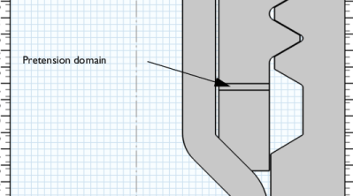
Click to expand the Object Selections section. Click to expand the Boundary Selections section. The selections listed in these sections are defined on the geometry in the Inventor assembly. For more details see Notes About the COMSOL Implementation.
Work Plane 1 (wp1)
1
In the Geometry toolbar, click  Work Plane.
2
In the Settings window for Work Plane, locate the Plane Definition section.
3
From the Plane list, choose zx-plane.
Add Component
In the Model Builder window, right-click the root node and choose Add Component>2D Axisymmetric.
Geometry 2
1
In the Settings window for Geometry, locate the Units section.
2
From the Length unit list, choose mm.
Cross Section 1 (cro1)
1
In the Geometry toolbar, click  Cross Section.
2
In the Settings window for Cross Section, locate the Selections of Resulting Entities section.
3
Select the Selections from 3D check box.
4
Click  Build Selected.
Union 1 (uni1)
1
In the Geometry toolbar, click  Booleans and Partitions and choose Union.
2
In the Settings window for Union, locate the Union section.
3
From the Input objects list, choose Male fitting (Cross Section 1).
Form Union (fin)
1
In the Model Builder window, under Component 2 (comp2)>Geometry 2 click Form Union (fin).
2
In the Settings window for Form Union/Assembly, locate the Form Union/Assembly section.
3
From the Action list, choose Form an assembly.
4
Clear the Create pairs check box.
Warning 1 (warning1)
In the Geometry toolbar, click  Build All.
Add Material
1
In the Home toolbar, click  Add Material to open the Add Material window.
2
Go to the Add Material window.
3
In the tree, select Built-in>Structural steel.
4
Right-click and choose Add to Component 2 (comp2).
5
In the Home toolbar, click  Add Material to close the Add Material window.
Add Physics
1
In the Home toolbar, click  Add Physics to open the Add Physics window.
2
Go to the Add Physics window.
3
In the tree, select Structural Mechanics>Solid Mechanics (solid).
4
Click Add to Component 2 in the window toolbar.
5
In the Home toolbar, click  Add Physics to close the Add Physics window.
Definitions (comp2)
Contact Pair 1 (p1)
1
In the Definitions toolbar, click  Pairs and choose Contact Pair.
2
In the Settings window for Pair, locate the Source Boundaries section.
3
From the Selection list, choose Faceset2.pipe (Cross Section 1).
4
Locate the Destination Boundaries section. From the Selection list, choose Faceset2.adaptor (Cross Section 1).
Contact Pair 2 (p2)
1
In the Definitions toolbar, click  Pairs and choose Contact Pair.
2
In the Settings window for Pair, locate the Source Boundaries section.
3
From the Selection list, choose Faceset1.housing (Cross Section 1).
4
Locate the Destination Boundaries section. From the Selection list, choose Faceset1.adaptor (Cross Section 1).
Contact Pair 3 (p3)
1
In the Definitions toolbar, click  Pairs and choose Contact Pair.
2
In the Settings window for Pair, locate the Source Boundaries section.
3
From the Selection list, choose Faceset2.housing (Cross Section 1).
4
Locate the Destination Boundaries section. From the Selection list, choose Faceset1.pipe (Cross Section 1).
Solid Mechanics (solid)
Contact 1a
1
In the Model Builder window, under Component 2 (comp2) right-click Solid Mechanics (solid) and choose Pairs>Contact.
2
In the Settings window for Contact, locate the Pair Selection section.
3
Under Pairs, click  Add.
4
In the Add dialog box, in the Pairs list, choose Contact Pair 1 (p1), Contact Pair 2 (p2), and Contact Pair 3 (p3).
5
6
In the Settings window for Contact, locate the Contact Method section.
7
From the Formulation list, choose Augmented Lagrangian.
Friction 1
1
In the Physics toolbar, click  Attributes and choose Friction.
2
In the Settings window for Friction, locate the Friction Parameters section.
3
In the μ text field, type mu.
4
Locate the Initial Value section. From the Previous contact state list, choose In contact.
Roller 1
1
In the Physics toolbar, click  Boundaries and choose Roller.
2
Global Definitions
Parameters 1
Continue with loading the parameters used for setting up the simulation.
1
In the Model Builder window, under Global Definitions click Parameters 1.
2
In the Settings window for Parameters, locate the Parameters section.
3
Click  Load from File.
4
Definitions (comp2)
Integration 1 (intop1)
1
In the Definitions toolbar, click  Nonlocal Couplings and choose Integration.
2
In the Settings window for Integration, locate the Source Selection section.
3
From the Selection list, choose Pre-tension domain (Cross Section 1).
4
Locate the Advanced section. From the Frame list, choose Material  (R, PHI, Z).
Solid Mechanics (solid)
1
Click the  Show More Options button in the Model Builder toolbar.
2
In the Show More Options dialog box, in the tree, select the check box for the node Physics>Equation-Based Contributions.
3
Global Equations 1
1
In the Physics toolbar, click  Global and choose Global Equations.
2
In the Settings window for Global Equations, locate the Global Equations section.
3
4
Locate the Units section. Click  Select Dependent Variable Quantity.
5
In the Physical Quantity dialog box, select Solid Mechanics>Strain tensor (1) in the tree.
6
7
In the Settings window for Global Equations, locate the Units section.
8
Click  Select Source Term Quantity.
9
In the Physical Quantity dialog box, select General>Force (N) in the tree.
10
Linear Elastic Material 1
In the Model Builder window, click Linear Elastic Material 1.
Initial Stress and Strain 1
1
In the Physics toolbar, click  Attributes and choose Initial Stress and Strain.
2
In the Settings window for Initial Stress and Strain, locate the Domain Selection section.
3
Click  Clear Selection.
4
From the Selection list, choose Pre-tension domain (Cross Section 1).
5
Locate the Initial Stress and Strain section. In the ε0 table, enter the following settings:
Spring Foundation 1
1
In the Physics toolbar, click  Boundaries and choose Spring Foundation.
2
3
In the Settings window for Spring Foundation, locate the Spring section.
4
5
In the kA table, enter the following settings:
Mesh 2
1
In the Model Builder window, under Component 2 (comp2) click Mesh 2.
2
In the Settings window for Mesh, locate the Sequence Type section.
3
From the list, choose User-controlled mesh.
Size 1
1
In the Model Builder window, right-click Free Triangular 1 and choose Size.
2
In the Settings window for Size, locate the Geometric Entity Selection section.
3
From the Geometric entity level list, choose Boundary.
4
From the Selection list, choose Faceset2.adaptor (Cross Section 1).
5
Locate the Element Size section. Click the Custom button.
6
Locate the Element Size Parameters section. Select the Maximum element size check box.
7
8
Click  Build All.
Add Study
1
In the Home toolbar, click  Add Study to open the Add Study window.
2
Go to the Add Study window.
3
Find the Studies subsection. In the Select Study tree, select General Studies>Stationary.
4
5
In the Home toolbar, click  Add Study to close the Add Study window.
Study 1
Step 1: Stationary
1
In the Settings window for Stationary, click to expand the Study Extensions section.
2
Select the Auxiliary sweep check box.
3
4
5
In the Model Builder window, click Study 1.
Solution 1 (sol1)
1
In the Study toolbar, click  Show Default Solver.
2
In the Model Builder window, expand the Solution 1 (sol1) node.
3
In the Model Builder window, expand the Study 1>Solver Configurations>Solution 1 (sol1)>Stationary Solver 1>Segregated 1 node, then click Solid Mechanics.
4
In the Settings window for Segregated Step, click to expand the Method and Termination section.
5
From the Termination technique list, choose Tolerance.
6
In the Study toolbar, click  Compute.
Results
Stress (solid)
The first automatically generated plot group contains a surface plot of the von Mises stress, and a line plot of the contact pressure.
Stress, 3D (solid)
To visualize the solution in 3D, a plot is also generated based on a revolution dataset.
Surface 1
1
In the Model Builder window, expand the Stress, 3D (solid) node, then click Surface 1.
2
In the Settings window for Surface, locate the Expression section.
3
From the Unit list, choose MPa.
Stress, 3D (solid)
1
In the Model Builder window, click Stress, 3D (solid).
2
In the Settings window for 3D Plot Group, locate the Color Legend section.
3
Select the Show maximum and minimum values check box.
The results plot should now appear similar to that in Figure 3