Two-Pole Three-Phase Induction Motor

Using a skewed squirrel cage in synchronous motors helps to reduce the rotor locking tendency. This locking tendency appears when the squirrel cage slots are under the stator windings, which cause magnetic attraction. Due to this nonsymmetrical design, a simulation to compute the motor torque needs to be performed either on the full motor geometry or on a 2D cross section for several angular positions of the rotor cage.

The geometry for this model is an assembly in PTC Creo Parametric. The assembly is transferred using the LiveLink interface to COMSOL Multiphysics, where the magnetic field is computed for 5 cross sections along the motor. Leveraging the selections defined with the LiveLink interface on the geometry in the PTC Creo Parametric it is straightforward to set up the simulation.

Figure 1: Plot of the magnetic flux density norm on a cross section along the motor displayed at the correct axial position on the 3D geometry.

Model Definition

The geometry of the three phase induction motor housing is shown in Figure 2 below.

Figure 2: The geometry of a three phase induction motor housing assembly.

The rotor consist of an iron core and an aluminum skewed squirrel cage. The cage is made of 24 bars with a tilt of 30 degrees/m.

Figure 3: Skewed squirrel cage geometry of the motor.

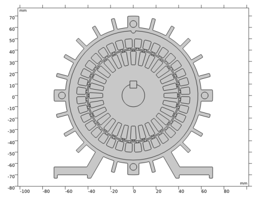
To reduce the computational time the simulation is solved on 2D cross sections, for example the cross section shown in Figure 4 in below.

Figure 4: 2D cross section of the induction motor.

Due to the skewed shape of the squirrel cage the problem is not symmetric. Thus we need to compute the magnetic field at several position along the axis of the motor and average the obtained results in order to get a better approximation. A parametric sweep is set up to automatically generate the 2D geometry and compute the solution at different positions.

The stator is made of 6 coils (single windings) with 3 slots per pole and phase, which make a total of 36 slots for a such a 2 pole pairs design. The stator core is made of soft iron and the stator coils are made of copper.

Figure 5: Windings of the 2 pairs pole three-phase induction motor.

A 0.01 A three-phase current is applied to the stator coil. The current supply frequency, f0, is 50 Hz. The angular speed of stator ωs is defined as:

where n is the number of pole pairs. This mean that the expected angular speed of stator is 157.08 Hz.

The slip in is defined as the ratio of the difference between the stator and rotor angular frequency relative to the stator angular frequency:

When the slip is null the rotor is rotating at the same speed as the stator field. When the slip is 1 the rotor is fixed.

In this model, a time-harmonic analysis is considered to compute the motor torque, the steel losses and the rotor losses. The implementation of a time-harmonic analysis for an induction problem is discussed in the model Frequency Domain Study of Three-Phase Motor available in the AC/DC Module’s Application Library. These model uses the approach of frozen rotor where the stator is excited at the slip angular frequency. The slip angular frequency is defined as

The model focus for a slip with the range between 0 and 5%. For such a design one can expect acceptable accuracy for qualitative analysis.

Not all the parts of the assembly are physically modeled, only the rotor and the cage, the rotor, and the coil are considered.

Results and Discussion

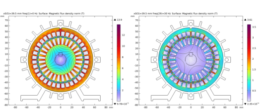
The figure Figure 6 below shows the norm magnetic field together with the contour distribution of the z-component of the vector potential at 0 and 5% slip.

Figure 6: Norm of the magnetic field (surface) and vector potential (contour), z-component, at 0 (left) and 5% slip (right).

The figure Figure 6 below shows the out-of-plane component of the current density at 0 and 5% slip.

Figure 7: Current density, z-component, at 0 (left) and 5% slip (right).

Since the analysis performed is in the frequency domain, the solution plotted in Figure 6 and Figure 7 are the real part of the norm of the magnetic field and the current density. It is possible to visualize the evolution of the fields during a cycle by changing the value of the phase in the dataset or by creating an animation using the dynamic data extension.

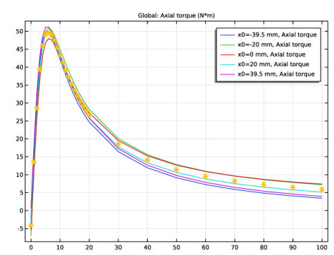
The figure Figure 8 below shows the torque versus the slip at several cut section in the motor. In dashed line the average value. As expected for an induction motor, the torque is null at the synchronous speed. Also a maximum is visible at a 0.3 % slip.One can notice the difference at between the torque value depending on the cage position in the motor. The difference can be at maximum 20% which is not negligible, he average value provide a closer solution to the reality.

Figure 8: Torque vs slip at 5 different cut section within the motor and average value (dashed).

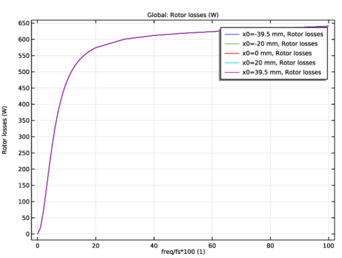
The figure Figure 9 below shows the rotor losses versus the slip at several cut section in the motor. As expected for an induction motor, the losses are minimum at the synchronous speed.

Figure 9: Rotor losses vs slip at 5 different cut section within the motor.

Notes About the COMSOL Implementation

The motor assembly is transferred from PTC Creo Parametric using the LiveLink interface. For assembly components that are important for the analysis setup, selections are defined on the CAD assembly in PTC Creo Parametric using the LiveLink interface. These selections are transfered together with the geometry to COMSOL Multiphysics, and they are also mapped to the geometry of the 2D cross section, simplifying the simulation setup. The selections defined in the PTC Creo Parametric file are listed in the table below.

Table 1: Material selections
Selection name	Part name
BOLTS	M6X165_.PRT
CASING_FAN	CASING_MAIN_.PRT CASING_SIDE_.PRT CASING_LEFT_.PRT
PHASE_A	STATOR_COIL_.PRT
PHASE_A_MINUS	STATOR_COIL_.PRT
PHASE_B	STATOR_COIL_2_.PRT
PHASE_B_MINUS	STATOR_COIL_2_.PRT
PHASE_C	STATOR_COIL_3_.PRT
PHASE_C_MINUS	STATOR_COIL_3_.PRT
ROTOR_COIL	ROTOR_COIL.PRT
ROTOR_CORE_SHAFT	ROTOR_CORE.prt SHAFT_.PRT KEY_80_.PRT
STATOR_CORE	STATOR_CORE_.PRT

The CAD assembly in PTC Creo Parametric is parameterized, and some key dimensional parameters have been modifiable from the simulation, so that a parametric sweep can be set up, although this currently not done in this tutorial. These parameters are listed in the table below.

Table 2: Parameters in CAD Package
CAD name	COMSOL name
AIR_GAP	LL_AIR_GAP
N_BARS	LL_N_BARS
N_POLES	LL_N_POLES
N_SLOT_PER_POLE	LL_N_SLOT_PER_POLE
R_ROTOR	LL_R_ROTOR
RA_STATOR	LL_RA_STATOR
RI_CAGE	LL_RI_CAGE

For a faster update of the plot combining results from the 2D simulation with the 3D geometry, displayed in Figure 1, a model method is used. The method updates the 3D representation of the geometry and the 2D solution for a specified cross section position.

LiveLink_for_PTC_Creo_Parametric/Tutorials,_LiveLink_Interface/induction_motor_llcreop

Modeling Instructions

In PTC Creo Parametric open the file induction_motor_cad/induction_motor.asm located in the model’s Application Library folder.

Switch to the COMSOL Desktop.

COMSOL Desktop

From the menu, choose .

In the window, click

In the window, click

Make sure that the CAD Import Module kernel is used.

In the window, under click .

In the window for , locate the section.

From the list, choose .

LiveLink for PTC Creo Parametric 1 (cad1)

In the toolbar, click

and choose .

In the window for , locate the section.

Click .

Global Definitions

Parameters 1

In the window, under click .

In the window for , locate the section.

In the table, enter the following settings:


Name	Expression	Value	Description
x0	0	0	Section cut position
f0	60[Hz]	60 Hz	Supply frequency
a0	1[mm^2]	1E-6 m²	Coil wire cross-section area
I_stat	5[A]	5 A	Coil wire current
fs	2*f0/LL_N_POLES	30 Hz	Synchronuous frequency
L	80[mm]	0.08 m	Motor length

Geometry 1

Work Plane 1 (wp1)

In the toolbar, click

In the window for , locate the section.

From the list, choose .

In the text field, type x0.

Adjacent Selection 1 (adjsel1)

In the toolbar, click

and choose .

In the window for , locate the section.

Click

In the dialog box, select in the list.

Click .

Form Union (fin)

In the window, under click .

In the window for , locate the section.

From the list, choose .

Clear the check box.

Mesh 1

Free Triangular 1

In the toolbar, click

and choose .

In the window for , locate the section.

From the list, choose .

Click

Add Component

In the window, right-click the root node and choose .

Geometry 2

In the window for , locate the section.

From the list, choose .

Cross Section 1 (cro1)

In the toolbar, click

In the window for , locate the section.

Select the check box.

From the list, choose .

Select the check box.

Click

Convert to Solid 1 (csol1)

In the toolbar, click

and choose .

In the window for , locate the section.

From the list, choose .

In the text field, type 1.0E-5.

Force Calculation Domain

In the toolbar, click

In the window for , type Force Calculation Domain in the text field.

Locate the section. In the text field, type LL_R_ROTOR.

Locate the section. Select the check box.

All_domains

In the toolbar, click

and choose .

In the window for , type All_domains in the text field.

Locate the section. From the list, choose .

Study_domains

In the toolbar, click

and choose .

In the window for , type Study_domains in the text field.

Locate the section. Click

In the dialog box, select in the list.

Click .

In the window for , locate the section.

Click

In the dialog box, in the list, choose and .

Click .

Form Union (fin)

In the window, click .

In the window for , click

Add Material

In the toolbar, click

to open the window.

Go to the window.

In the tree, select .

Right-click and choose .

In the tree, select .

Right-click and choose .

In the tree, select .

Right-click and choose .

In the toolbar, click

to close the window.

Global Definitions

Structural steel (mat3)

In the window for , locate the section.

In the table, enter the following settings:


Property	Variable	Value	Unit	Property group
Relative permeability	mur_iso ; murii = mur_iso, murij = 0	1000	1	Basic
Electrical conductivity	sigma_iso ; sigmaii = sigma_iso, sigmaij = 0	0[S/m]	S/m	Basic
Relative permittivity	epsilonr_iso ; epsilonrii = epsilonr_iso, epsilonrij = 0	1	1	Basic