PDF

Drying of a Potato Sample
Introduction
Drying of porous media is an important process in the food and paper industry among others. Many physical effects must be considered: fluid flow, heat transfer with phase change, and transport of participating liquids and gases. All of these effects are strongly coupled, and predefined interfaces can be used to model these effects in an hygroscopic porous medium with COMSOL Multiphysics.
In this model, the liquid and gaseous phases are assumed to be in equilibrium inside a potato sample modeled as a porous medium, and the changing water saturation is computed over time, to model the heat and moisture transport by a two-phase flow.
Model Definition
This model describes a laminar dry airflow through a potato sample, modeled as a porous medium containing moist air and liquid water. The geometry and principle is shown in Figure 1.
Figure 1: Geometry and principle of the model.
Heat and Moisture Transport in Air
In the moist air domain, it is assumed that no liquid water is present. This means that all the moisture leaves the porous medium under vapor state.
The transport and thermodynamic properties of air with water vapor can be described using mixture laws, based on the amount of water vapor and dry air. This is done automatically in the Moist Air feature and subfeature in the Heat Transfer interface. See the Heat Transfer Module User’s Guide for the governing equations. As the input term for water vapor, the relative humidity from the moisture transport equation is used in the Heat Transfer and Fluid Flow interfaces.
The compressible Navier–Stokes equations are solved to compute the velocity and pressure fields of the free flow for the convective transport of heat and moisture.
Another relevant effect for the moisture transport is the binary diffusion of vapor and air. The variations of the density of moist air induced by vapor transport are relatively small in the current configuration, so the diluted species formulation is used.
Two phase flow in The Potato Sample
The basic principle of modeling two phase flow in porous media is similar for many applications. First, to account for different phases, saturation variables are used that fulfill the following constraint:
(1)
where the index g is used for the gaseous phase (which in this model is moist air) and the index l is used for the liquid phase (which in this model is water).
Single-phase flow in porous media is described by the Brinkman Equations. With an additional liquid phase, capillary effects also arise and the liquid flow is driven by a pressure gradient and capillary pressure pc = pg − pl. How to deal with the latter one depends on the application: sometimes the capillary pressure can be neglected, sometimes it is the driving effect and different approaches exist.
In this model, the capillary effects are treated by an additional diffusion term in the transport equation. The Brinkman Equation is used to calculate the flow field ug and pressure distribution pg of moist air in the porous medium. Therefore the porosity εp must take into account that only a fraction of the void space is occupied by the gas phase.
The liquid phase velocity is small compared to the moist air velocity and such that Darcy’s law is defined in terms of the gas phase pressure gradient to calculate the water velocity ul according to
(2)
where κl and μl are the permeability and viscosity of the liquid phase.
Finally, due to the dimensions of the porous medium, the gravity effects on transport are neglected in both phases.
Moisture Transport in The Potato Sample
Following the ideas about mechanistic formulations from (Ref. 1), and by summing the mass conservation equations for vapor and liquid water, a single equation can be written to calculate the time dependent evolution of moisture content, , in the porous medium:
(3)
The total moisture content accounts for the vapor and liquid water in the pores of the medium:
with ρl the liquid water density, ρg the moist air density, and ωv the vapor mass fraction defined as:
The remaining terms in Equation 3 account for:
A common correlation for the effective diffusivity Deff in an unsaturated medium is the Millington and Quirk equation:
with the vapor-air diffusivity Dva = 2.6105 m2/s.
Convection of liquid water due to total pressure gradient, with the flow field ul computed by the Darcy’s Law in Equation 2. The permeability for the liquid phase κl depends on the overall permeability of the porous matrix κ and a relative permeability (see Permeability) κrl.
with the diffusion coefficient Dw defined as (Ref. 1):
with ρs the solid phase density.
When summing the conservation equations to obtain Equation 3, the condensation source term in the mass conservation equation for liquid water cancels out with the evaporation source term in the mass conservation equation for vapor. However, the evaporation source can be expressed as follows:
Heat Transfer
Inside the porous domain the overall velocity field for liquid and gaseous phase contributes to the heat convection term. It is possible to account for the liquid water and moist air phases, by using the liquid saturation calculated by the moisture transport equation.
The mixture law is applicable in the gaseous phase, and averaged thermal properties (ρCp)eff and keff are defined by taking into account the properties of the porous matrix (ρs, Cp,s, ks), moist air (ρg, Cp,g, kg), and liquid water (ρl, Cp,l, kl):
(4)
Then the overall velocity can be expressed as the average of moist air and liquid water velocity, which is
(5)
The diffusive flux of enthalpy, due to vapor diffusion in air, and the capillary flux, due to the presence of the liquid water in the pores, are included in the following heat source term:
(6)
The heat of evaporation is inserted as a source term in the heat transfer equation according to
(7)
where Lv (J/mol) is the latent heat of evaporation.
Permeability
The permeability of the porous matrix κ defines the absolute permeability. When two phases are present, the permeability of each phase depends also on the saturation. This is defined by the relative permeabilities κrl and κrg for liquid and gaseous phase respectively, so that κl = κκrl and κg = κκrg. The determination of relative permeability curves is often done empirically or experimentally and the form strongly depends on the porous material properties and the liquids themselves. The functions that are used in this model (Ref. 2) are defined such that they are always positive:
The variable sli is the irreducible liquid phase saturation, describing the saturation of the liquid phase that will remain inside the porous medium.
Results and Discussion
Inside the potato sample, the relative humidity decreases from about 100% everywhere at the beginning of the simulation to about 10% at the end, which is the ambient air condition (Figure 2 and Figure 3).
Figure 2: Relative humidity after 5000 s.
At the beginning of the simulation (time 5000 s), the vapor concentration is close to its saturation value in the moist air enclosed in the pores. It goes down to the ambient concentration towards the end of the simulation.
Figure 3: Relative humidity after 40,000 s.
Because moisture is composed of vapor and liquid water in the porous medium, a good quantifier of the drying process is the liquid saturation. Figure 4 shows the drying front in the porous medium at time 5000 s, starting from the top-left corner, which is facing the dry air flow.
Figure 4: Liquid saturation after 5000 s.
The temperature plot (Figure 5) shows the corresponding cooling in the potato sample at time 5000 s, due to evaporation of the liquid water close to the drying front.
Figure 5: Temperature field after 5000 s.
Finally, the evolution of the moisture content in the potato sample over time is shown below.
Figure 6: Moisture content in the potato sample over time.
Notes About the COMSOL Implementation
Using a proper mesh size is important to resolve the steep gradients at the interface boundaries. Therefore the default mesh is refined.
To get good convergence of the time dependent behavior, first solve the stationary flow equations only. This solution will then be used for the time dependent study step. This approximation neglects the evaporation mass source in the fluid flow computation.
References
1. A.K. Datta, “Porous media approaches to studying simultaneous heat and mass transfer in food processes. I: Problem formulations,” Journal of Food Engineering, vol. 80, 2007.
2. A.K. Datta, “Porous media approaches to studying simultaneous heat and mass transfer in food processes. II: Property data and representative results,” Journal of Food Engineering, vol. 80, 2007.
3. A. Halder, A. Dhall, and A.K. Datta, “Modeling Transport in Porous Media with Phase Change: Applications to Food Processing,” J. Heat Transfer, vol. 133, no. 3, 2011.
Application Library path: Heat_Transfer_Module/Phase_Change/potato_drying
Modeling Instructions
From the File menu, choose New.
New
In the New window, click  Model Wizard.
Model Wizard
1
In the Model Wizard window, click  2D.
2
In the Select Physics tree, select Heat Transfer>Heat and Moisture Transport>Heat and Moisture Flow>Laminar Flow.
3
Click Add.
4
Click  Study.
5
In the Select Study tree, select General Studies>Time Dependent.
6
For this model, some parameters are needed. Start by loading all of them from a text file.
Global Definitions
Parameters 1
1
In the Model Builder window, under Global Definitions click Parameters 1.
2
In the Settings window for Parameters, locate the Parameters section.
3
Click  Load from File.
4
Define the relative permeabilities for water vapor and liquid water as functions of liquid water saturation. The advantage of using functions is that they can be plotted immediately.
Definitions
Relative Permeability, Moist Air
1
In the Model Builder window, expand the Component 1 (comp1)>Definitions node.
2
Right-click Definitions and choose Functions>Piecewise.
3
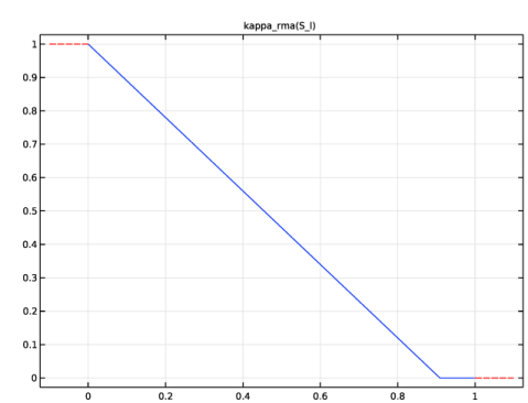
In the Settings window for Piecewise, type Relative Permeability, Moist Air in the Label text field.
4
In the Function name text field, type kappa_rma.
5
Locate the Definition section. In the Argument text field, type S_l.
6
Find the Intervals subsection. In the table, enter the following settings:
To force the saturation to be always positive eps is used as minimum value.
7
Relative Permeability, Liquid Phase
1
In the Home toolbar, click  Functions and choose Global>Piecewise.
2
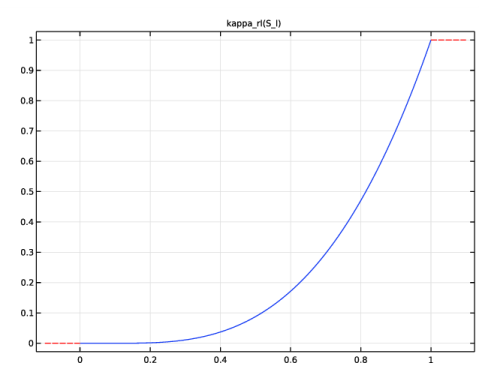
In the Settings window for Piecewise, type Relative Permeability, Liquid Phase in the Label text field.
3
In the Function name text field, type kappa_rl.
4
Locate the Definition section. In the Argument text field, type S_l.
5
Find the Intervals subsection. In the table, enter the following settings:
6
Define the sorption isotherm by interpolation of tabulated data.
Sorption Isotherm
1
In the Home toolbar, click  Functions and choose Local>Interpolation.
2
In the Settings window for Interpolation, type Sorption Isotherm in the Label text field.
3
Locate the Definition section. In the Function name text field, type wc_int.
4
Click  Load from File.
5
6
Locate the Units section. In the Argument table, enter the following settings:
7
In the Function table, enter the following settings:
8
Now, define the geometry.
Geometry 1
Rectangle 1 (r1)
1
In the Geometry toolbar, click  Rectangle.
2
In the Settings window for Rectangle, locate the Size and Shape section.
3
In the Width text field, type 0.15.
4
In the Height text field, type 0.05.
Rectangle 2 (r2)
1
In the Geometry toolbar, click  Rectangle.
2
In the Settings window for Rectangle, locate the Size and Shape section.
3
In the Width text field, type 0.04.
4
In the Height text field, type 0.005.
5
Locate the Position section. In the x text field, type 0.04.
Fillet 1 (fil1)
1
In the Geometry toolbar, click  Fillet.
2
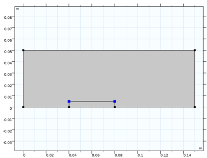
On the object r2, select Points 3 and 4 only.
It might be easier to select the points by using the Selection List window. To open this window, in the Home toolbar click Windows and choose Selection List. (If you are running the cross-platform desktop, you find Windows in the main menu.)
3
In the Settings window for Fillet, locate the Radius section.
4
In the Radius text field, type 2e-3.
5
In the Geometry toolbar, click  Build All.
Definitions
Define the ambient conditions used later in the domain and boundary conditions.
Ambient Properties 1 (ampr1)
1
In the Physics toolbar, click  Shared Properties and choose Ambient Properties.
2
In the Settings window for Ambient Properties, locate the Ambient Conditions section.
3
In the Tamb text field, type T0.
4
In the φamb text field, type phi_0.
Heat Transfer in Moist Air (ht)
Define the domain and boundary conditions for each interface. Start with the Heat Transfer in Moist Air interface, by setting the initial and boundary conditions, and by adding a Moist Porous Medium domain condition.
Initial Values 1
Use the ambient temperature defined previously as input.
1
In the Model Builder window, under Component 1 (comp1)>Heat Transfer in Moist Air (ht) click Initial Values 1.
2
In the Settings window for Initial Values, locate the Initial Values section.
3
From the T list, choose Ambient temperature (ampr1).
Moist Porous Medium 1
1
In the Physics toolbar, click  Domains and choose Moist Porous Medium.
2
Porous Matrix 1
1
In the Model Builder window, click Porous Matrix 1.
2
In the Settings window for Porous Matrix, locate the Matrix Properties section.
3
From the Define list, choose Solid phase properties.
Inflow 1
1
In the Physics toolbar, click  Boundaries and choose Inflow.
2
3
In the Settings window for Inflow, locate the Upstream Properties section.
4
From the Tustr list, choose Ambient temperature (ampr1).
Outflow 1
1
In the Physics toolbar, click  Boundaries and choose Outflow.
2
Laminar Flow (spf)
Continue with the Laminar Flow interface.
1
In the Model Builder window, under Component 1 (comp1) click Laminar Flow (spf).
2
In the Settings window for Laminar Flow, locate the Physical Model section.
3
From the Compressibility list, choose Compressible flow (Ma<0.3).
The next step enables additional features for the flow interface to account for porous domains also.
4
Select the Enable porous media domains check box.
Porous Medium 1
1
In the Physics toolbar, click  Domains and choose Porous Medium.
2
Porous Matrix 1
Set the material properties for the definition of Brinkman equation for vapor phase.
1
In the Model Builder window, expand the Porous Medium 1 node, then click Porous Matrix 1.
2
In the Settings window for Porous Matrix, locate the Matrix Properties section.
3
From the εp list, choose User defined. In the associated text field, type por*(1-mt.sl).
The pore space is partially filled with liquid water, so that the available space for water vapor depends on the porosity and the saturation.
4
From the κ list, choose User defined. In the associated text field, type kappa_rma(mt.sl)*kappa.
Inlet 1
1
In the Physics toolbar, click  Boundaries and choose Inlet.
2
3
In the Settings window for Inlet, locate the Boundary Condition section.
4
From the list, choose Fully developed flow.
5
Locate the Fully Developed Flow section. In the Uav text field, type u0.
Outlet 1
1
In the Physics toolbar, click  Boundaries and choose Outlet.
2
Moisture Transport in Air (mt)
Finally, set the domain, initial, and boundary conditions for the Moisture Transport in Air interface.
Initial Values 1
1
In the Model Builder window, under Component 1 (comp1)>Moisture Transport in Air (mt) click Initial Values 1.
2
In the Settings window for Initial Values, locate the Initial Values section.
3
From the φw,0 list, choose Ambient relative humidity (ampr1).
Hygroscopic Porous Medium 1
1
In the Physics toolbar, click  Domains and choose Hygroscopic Porous Medium.
2
3
In the Settings window for Hygroscopic Porous Medium, locate the Moisture Transport Properties section.
4
From the Capillary model list, choose Diffusion.
Liquid Water 1
1
In the Model Builder window, expand the Hygroscopic Porous Medium 1 node, then click Liquid Water 1.
2
In the Settings window for Liquid Water, locate the Liquid Water Properties section.
3
In the κrl text field, type kappa_rl(mt.sl).
Initial Values 2
1
In the Physics toolbar, click  Domains and choose Initial Values.
2
3
In the Settings window for Initial Values, locate the Initial Values section.
4
In the φw,0 text field, type phi_1.
Inflow 1
1
In the Physics toolbar, click  Boundaries and choose Inflow.
2
3
In the Settings window for Inflow, locate the Upstream Properties section.
4
From the Tustr list, choose Ambient temperature (ampr1).
5
From the φw,ustr list, choose Ambient relative humidity (ampr1).
Outflow 1
1
In the Physics toolbar, click  Boundaries and choose Outflow.
2
Materials
Next, define the hygrothermal properties for the porous medium, based on measured data for potato.
Potato
1
In the Model Builder window, under Component 1 (comp1) right-click Materials and choose More Materials>Porous Material.
2
In the Settings window for Porous Material, type Potato in the Label text field.
3
Add the Solid subnode and define its material properties.
4
Locate the Phase-Specific Properties section. Click  Add Required Phase Nodes.
Solid 1 (pmat1.solid1)
1
In the Model Builder window, click Solid 1 (pmat1.solid1).
2
In the Settings window for Solid, locate the Solid Properties section.
3
In the θs text field, type 1-por.
4
Locate the Material Contents section. In the table, enter the following settings:
Potato (pmat1)
Set the remaining material properties in the Homogenized Properties section.
1
In the Model Builder window, click Potato (pmat1).
2
In the Settings window for Porous Material, locate the Homogenized Properties section.
3
As the water content is defined as a function of the relative humidity, add the relative humidity as a model input required by the material.
4
In the Model Builder window, click Basic (def).
5
In the Settings window for Basic, locate the Model Inputs section.
6
Click  Select Quantity.
7
In the Physical Quantity dialog box, type relative in the text field.
8
In the tree, select General>Relative humidity (1).
9
Definitions (comp1)
Define an integration operator in the porous domain, in order to check the moisture content evolution.
Integration Porous Medium
1
In the Definitions toolbar, click  Nonlocal Couplings and choose Integration.
2
3
In the Settings window for Integration, type Integration Porous Medium in the Label text field.
4
In the Operator name text field, type intopPorous.
To resolve all effects and get a better convergence for this highly nonlinear problem, refine the mesh to resolve the interface properly.
Mesh 1
1
In the Model Builder window, under Component 1 (comp1) click Mesh 1.
2
In the Settings window for Mesh, locate the Physics-Controlled Mesh section.
3
From the Element size list, choose Extra fine.
4
Click  Build All.
Study 1
Add a stationary step that solves for the fluid flow only. This approximation does not account for the evaporation mass source in the porous medium for the fluid flow initialization. The solution is used for the computation of the time dependent solution of all the processes.
Stationary
1
In the Study toolbar, click  Study Steps and choose Stationary>Stationary.
2
Drag and drop above Step 2: Time Dependent.
3
In the Settings window for Stationary, locate the Physics and Variables Selection section.
4
In the table, clear the Solve for check boxes for Moisture Transport in Air (mt) and Heat Transfer in Moist Air (ht).
Step 2: Time Dependent
1
In the Model Builder window, click Step 2: Time Dependent.
2
In the Settings window for Time Dependent, locate the Study Settings section.
3
In the Output times text field, type range(0,10,90) range(100,100,900) range(1000,1000,40000).
Reduce the solver tolerance to enhance accuracy on mass balance.
4
From the Tolerance list, choose User controlled.
5
In the Relative tolerance text field, type 0.001.
6
In the Study toolbar, click  Compute.
Results
The default plots show the velocity, the pressure, the relative humidity (Figure 3), and the temperature.
Relative Humidity (mt)
Change the plot time to 5000 s for the relative humidity and the temperature to obtain Figure 2 and Figure 5.
1
In the Model Builder window, click Relative Humidity (mt).
2
In the Settings window for 2D Plot Group, locate the Data section.
3
From the Time (s) list, choose 5000.
4
In the Relative Humidity (mt) toolbar, click  Plot.
Temperature (ht)
1
In the Model Builder window, click Temperature (ht).
2
In the Settings window for 2D Plot Group, locate the Data section.
3
From the Time (s) list, choose 5000.
4
In the Temperature (ht) toolbar, click  Plot.
Liquid Saturation
Follow the instructions below to plot the liquid saturation in the porous medium at time 5000 s as in Figure 4, in order to check the evolution of the drying front.
1
In the Home toolbar, click  Add Plot Group and choose 2D Plot Group.
2
In the Settings window for 2D Plot Group, type Liquid Saturation in the Label text field.
3
Locate the Data section. From the Time (s) list, choose 5000.
Surface 1
1
Right-click Liquid Saturation and choose Surface.
2
In the Settings window for Surface, locate the Expression section.
3
In the Expression text field, type mt.sl.
4
In the Liquid Saturation toolbar, click  Plot.
Moisture Content in Porous Medium over Time
Follow the instructions below to plot the evolution of the moisture content over time in the porous medium as in Figure 6, in order to check the efficiency of the drying process.
1
In the Home toolbar, click  Add Plot Group and choose 1D Plot Group.
2
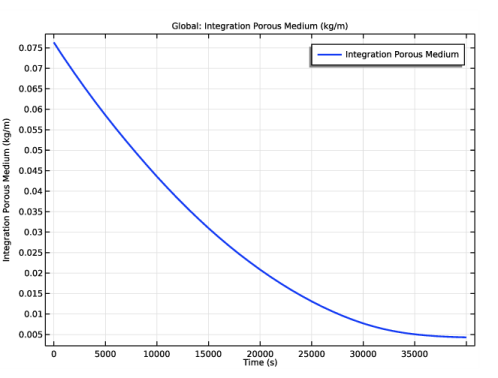
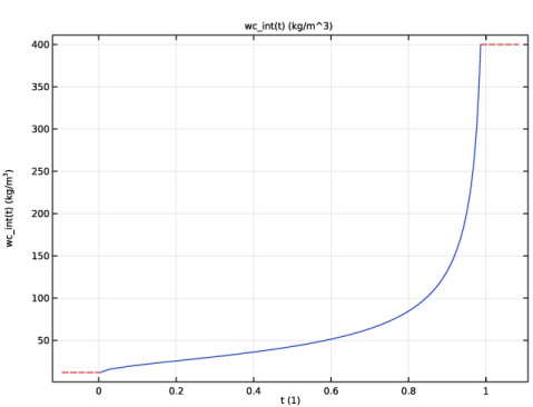
In the Settings window for 1D Plot Group, type Moisture Content in Porous Medium over Time in the Label text field.
Global 1
1
Right-click Moisture Content in Porous Medium over Time and choose Global.
2
In the Settings window for Global, locate the y-Axis Data section.
3
4
Click to expand the Coloring and Style section. In the Width text field, type 2.
5
In the Moisture Content in Porous Medium over Time toolbar, click  Plot.
Mass Balance
Finally, follow the instructions below to check the overall mass balance over time.
1
In the Results toolbar, click  Global Evaluation.
2
In the Settings window for Global Evaluation, type Mass Balance in the Label text field.
3
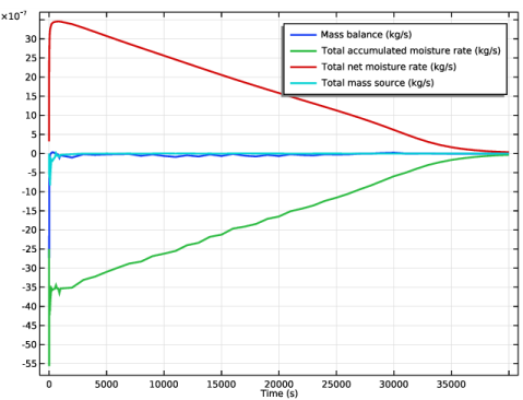
Click Replace Expression in the upper-right corner of the Expressions section. From the menu, choose Component 1 (comp1)>Moisture Transport in Air>Mass balance>mt.massBalance - Mass balance - kg/s.
4
Click Add Expression in the upper-right corner of the Expressions section. From the menu, choose Component 1 (comp1)>Moisture Transport in Air>Mass balance>mt.dwcInt - Total accumulated moisture rate - kg/s.
5
Click Add Expression in the upper-right corner of the Expressions section. From the menu, choose Component 1 (comp1)>Moisture Transport in Air>Mass balance>mt.ntfluxInt - Total net moisture rate - kg/s.
6
Click Add Expression in the upper-right corner of the Expressions section. From the menu, choose Component 1 (comp1)>Moisture Transport in Air>Mass balance>mt.GInt - Total mass source - kg/s.
7
Click  Evaluate.
Table
1
Go to the Table window.
2
Click Table Graph in the window toolbar.
Results
Mass Balance
1
In the Model Builder window, under Results click 1D Plot Group 8.
2
In the Settings window for 1D Plot Group, type Mass Balance in the Label text field.
Table Graph 1
1
In the Model Builder window, click Table Graph 1.
2
In the Settings window for Table Graph, click to expand the Legends section.
3
Select the Show legends check box.
4
Locate the Coloring and Style section. In the Width text field, type 2.