PDF

Freeze-Drying
Introduction
Freeze-drying, or lyophilization, is a dehydration process that is often used to preserve a perishable food or material. It is also frequently used as a way to remove water from goods, making them lighter and easier to transport. Lyophilization is widely recognized as an important technique in many industries. It is used, for example, in the pharmaceutical industry for the preservation of antibiotics, in the manufacturing of semiconductor ceramics, and by preservation initiatives, such as in the restoration of water-damaged documents. And of course, the process is widely used in the food industry, to preserve tasty snacks that can last up to 30 years. The wet substance is frozen and ice (or some other frozen solvent) is removed through sublimation in the presence of a high vacuum.
Freeze-drying relies on sublimation, where a frozen liquid undergoes phase change directly from a frozen state and into a gaseous state. As can be shown in a phase diagram, at very low pressures and temperatures, a solid can pass directly into the gaseous stage without passing through the intermediary liquid phase.
This model demonstrates the process of ice sublimation in a vial under vacuum-chamber conditions, a test case for many freeze-drying setups.
Model Definition
In this example, you model the process of sublimation of ice through the pores of a porous medium in a vial. Figure 1 depicts the model geometry cut in half.
Figure 1: Vial model geometry.
Since the geometry and boundary conditions are axisymmetric, a 2D axisymmetric model would be sufficient. However, for demonstration purposes and to make the model more general, a good compromise considering the computation time is to solve the model in 3D with a symmetry on the y = 0 plane.
Mass Transfer
The frozen product (here skim milk) initially fills 98% of the vial.The remaining gap contains the dried product and the vapor generated by sublimation, and expands during the sublimation process.The inert gas is neglected in the simulation.
The vapor flow rate Qm through the pores of the dried product is defined by the stationary Darcy’s law:
(1)
where ρv is the vapor density, μv is the vapor dynamic viscosity, pv is the vapor partial pressure, and κ is the permeability of the dried product.
The top of the vial is close to vacuum, maintained at a vapor pressure p0 of 24 Pa.
At the sublimation interface, the mass flux N0 is:
(2)
where ρice is the ice density, ε is the porosity of the product, and Vs is the sublimation interface velocity.
Heat Transfer
You solve the heat transfer equation for porous media, without convection in the frozen domain,
(3)
and with convection in the dried domain
(4)
Here, (ρCp)eff,dr and keff,dr refer to the equivalent volumetric heat capacity and thermal conductivity of the dried region, (ρCp)eff,fr and keff,fr refer to the equivalent volumetric heat capacity and thermal conductivity of the frozen region, Cp,v is the specific heat capacity of vapor, and u is the velocity obtained from Darcy’s law.
In the vapor domain, the density is calculated using the molar mass of vapor, Mv, and the ideal gas law:
(5)
where R is the universal gas constant.
Convective exchanges with the surrounding air occur all around the vial. At the bottom of the vial, convective exchanges with the shelf occur as well, and the heat transfer coefficient is lower on the center than on the exterior of the vial due to an air gap.
Ice-Vapor Interface
Assuming thermodynamic equilibrium at the phase change interface, the sublimation front temperature Ts is defined from the vapor pressure pv at this boundary, using the Clausius–Clapeyron relation:
(6)
where Ls is the sublimation latent heat.
Simultaneous heat and mass balances at the sublimation interface lead to the Stefan condition for the interface velocity Vs:
(7)
where Qs is the jump in the normal heat flux at the interface.
Results
The process of primary drying takes about 10 hours to transform most of the initial amount of ice. The frozen product has the proportions shown in Figure 2.
Figure 2: Temperature and heat flux at the end of the drying time period.
You can see from this visualization that the sublimation front has a concave curved shape that is lower around the outside edges of the vial wall. As the ice becomes a vapor, the mass of the solid decreases and therefore the mesh in the frozen domain squeezes as well.
Notes About the COMSOL Implementation
To set up the application in COMSOL Multiphysics, use the Deformed Geometry interface to track the ice surface, and then compute coupled mass and heat balances on the moving mesh. Figure 3 shows the initial mesh and Figure 4 shows the deformed mesh at the end of the simulation.
Figure 3: Initial swept mesh.
Figure 4: Deformed mesh at the end of the simulation.
In Equation 7, Qs corresponds to the jump in the normal heat flux at the interface. This quantity can be precisely evaluated through the Lagrange multiplier for temperature, T_lm. This variable is computed in the Phase Change Interface feature, which sets a fixed temperature weak constraint on the sublimation front.
References
1. A. Alonso and others, “Time-scale modeling and optimal control of freeze-drying,” Journal of Food Engineering, vol. 111, pp. 655–666, 2012.
2. W.J. Mascarenhas, H.U. Akay, and M.J. Pikal, “A computational model for finite element analysis of the freeze-drying process,” Computer Methods on Applied Mechanics and Engineering, vol. 148, pp. 105–124, 1997.
3. Hriberšek and others, “Lyophilization model of mannitol water solution in a laboratory scale lyophilizer”, Journal of Drug Delivery Science and Technology, vol. 45, pp. 28–38, 2018.
Application Library path: Heat_Transfer_Module/Phase_Change/freeze_drying
Modeling Instructions
From the File menu, choose New.
New
In the New window, click  Model Wizard.
Model Wizard
1
In the Model Wizard window, click  3D.
2
In the Select Physics tree, select Fluid Flow>Porous Media and Subsurface Flow>Darcy’s Law (dl).
3
Click Add.
4
In the Select Physics tree, select Heat Transfer>Porous Media>Heat Transfer in Porous Media (ht).
5
Click Add.
6
In the Select Physics tree, select Mathematics>Deformed Mesh>Legacy Deformed Mesh>Deformed Geometry (dg).
7
Click Add.
8
Click  Study.
9
In the Select Study tree, select General Studies>Time Dependent.
10
For this model, some parameters are needed. Start by loading all of them from a text file.
Global Definitions
Parameters 1
1
In the Model Builder window, under Global Definitions click Parameters 1.
2
In the Settings window for Parameters, locate the Parameters section.
3
Click  Load from File.
4
Add empty materials that will be linked later to the porous materials.
Vapor
1
In the Model Builder window, under Global Definitions right-click Materials and choose Blank Material.
2
In the Settings window for Material, type Vapor in the Label text field.
Ice
1
Right-click Materials and choose Blank Material.
2
In the Settings window for Material, type Ice in the Label text field.
Product (Skim Milk)
1
Right-click Materials and choose Blank Material.
2
In the Settings window for Material, type Product (Skim Milk) in the Label text field.
Geometry 1
1
In the Model Builder window, under Component 1 (comp1) click Geometry 1.
2
In the Settings window for Geometry, locate the Units section.
3
From the Length unit list, choose mm.
Cylinder 1 (cyl1)
1
In the Geometry toolbar, click  Cylinder.
2
In the Settings window for Cylinder, locate the Size and Shape section.
3
In the Radius text field, type R0.
4
In the Height text field, type Z0.
5
Click to expand the Layers section. In the table, enter the following settings:
6
Clear the Layers on side check box.
7
Select the Layers on top check box.
Cylinder 2 (cyl2)
1
In the Geometry toolbar, click  Cylinder.
2
In the Settings window for Cylinder, locate the Size and Shape section.
3
In the Radius text field, type R0.
4
In the Height text field, type Z0.
5
Locate the Layers section. In the table, enter the following settings:
Block 1 (blk1)
1
In the Geometry toolbar, click  Block.
2
In the Settings window for Block, locate the Size and Shape section.
3
In the Width text field, type R0*5.
4
In the Depth text field, type R0*2.
5
In the Height text field, type Z0.
6
Locate the Position section. In the x text field, type -R0*2.
7
In the y text field, type -R0*2.
Difference 1 (dif1)
1
In the Geometry toolbar, click  Booleans and Partitions and choose Difference.
2
In the Settings window for Difference, locate the Difference section.
3
Click  Paste Selection.
4
In the Paste Selection dialog box, type cyl1 cyl2 in the Selection text field.
5
6
In the Settings window for Difference, locate the Difference section.
7
Find the Objects to subtract subsection. Click to select the  Activate Selection toggle button.
8
9
Click  Build All Objects.
10
Click the  Zoom Extents button in the Graphics toolbar.
These steps create a geometry similar to that in Figure 1.
Definitions
Interface
1
In the Model Builder window, expand the Component 1 (comp1)>Definitions node.
2
Right-click Definitions and choose Variables.
Define the sublimation temperature at the phase change interface according to the Clausius-Clapeyron equation.
3
In the Settings window for Variables, type Interface in the Label text field.
4
Locate the Variables section. In the table, enter the following settings:
Integration 1 (intop1)
1
In the Definitions toolbar, click  Nonlocal Couplings and choose Integration.
2
In the Settings window for Integration, locate the Source Selection section.
3
Click  Paste Selection.
4
In the Paste Selection dialog box, type 1 3 5 in the Selection text field.
5
Minimum 1 (minop1)
1
In the Definitions toolbar, click  Nonlocal Couplings and choose Minimum.
2
In the Settings window for Minimum, locate the Source Selection section.
3
From the Geometric entity level list, choose Boundary.
4
Click  Paste Selection.
5
In the Paste Selection dialog box, type 6 13 20 in the Selection text field.
6
Add porous materials to the materials node, but do not define their properties at this point. After setting up the physics interface, COMSOL Multiphysics automatically detects which material properties are needed.
Materials
Porous Material 1 (pmat1)
In the Model Builder window, under Component 1 (comp1) right-click Materials and choose More Materials>Porous Material.
Porous Material 2 (pmat2)
1
Right-click Materials and choose More Materials>Porous Material.
2
Now, set up the physics interfaces. Start with the Darcy’s law interface, that simulates the vapor flow through the pores of the dried layer.
3
Click the  Show More Options button in the Model Builder toolbar.
4
In the Show More Options dialog box, in the tree, select the check box for the node Physics>Advanced Physics Options.
5
Darcy’s Law (dl)
1
In the Model Builder window, under Component 1 (comp1) click Darcy’s Law (dl).
2
3
In the Settings window for Darcy’s Law, click to expand the Equation section.
4
From the Equation form list, choose Stationary.
5
Locate the Physical Model section. In the pref text field, type 0.
6
Click to expand the Discretization section. Select the Compute boundary fluxes check box.
7
Fluid 1
1
In the Model Builder window, under Component 1 (comp1)>Darcy’s Law (dl)>Porous Medium 1 click Fluid 1.
2
In the Settings window for Fluid, locate the Fluid Properties section.
3
From the Fluid type list, choose Ideal gas.
4
From the Gas constant type list, choose Mean molar mass.
Initial Values 1
1
In the Model Builder window, under Component 1 (comp1)>Darcy’s Law (dl) click Initial Values 1.
2
In the Settings window for Initial Values, locate the Initial Values section.
3
In the p text field, type Pc.
Pressure 1
1
In the Physics toolbar, click  Boundaries and choose Pressure.
2
3
In the Settings window for Pressure, locate the Pressure section.
4
In the p0 text field, type Pc.
Mass Flux 1
1
In the Physics toolbar, click  Boundaries and choose Mass Flux.
2
3
In the Settings window for Mass Flux, locate the Mass Flux section.
4
In the N0 text field, type -ht.pci1.vn*rho_ice*por_p.
Symmetry 1
1
In the Physics toolbar, click  Boundaries and choose Symmetry.
2
Heat Transfer in Porous Media (ht)
Now, set up the Heat Transfer in Porous Media interface, in both dried and frozen layers.
Dried Layer
1
In the Model Builder window, under Component 1 (comp1)>Heat Transfer in Porous Media (ht) right-click Porous Medium 1 and choose Rename.
2
In the Rename Porous Medium dialog box, type Dried Layer in the New label text field.
3
Fluid 1
1
In the Model Builder window, click Fluid 1.
2
In the Settings window for Fluid, locate the Heat Convection section.
3
From the u list, choose Darcy’s velocity field (dl/porous1).
4
Locate the Thermodynamics, Fluid section. From the Fluid type list, choose Ideal gas.
5
From the Gas constant type list, choose Mean molar mass.
Porous Matrix 1
1
In the Model Builder window, click Porous Matrix 1.
2
In the Settings window for Porous Matrix, locate the Matrix Properties section.
3
From the Define list, choose Solid phase properties.
Initial Values 1
1
In the Model Builder window, under Component 1 (comp1)>Heat Transfer in Porous Media (ht) click Initial Values 1.
2
In the Settings window for Initial Values, locate the Initial Values section.
3
In the T text field, type Ti.
Frozen Layer
1
In the Physics toolbar, click  Domains and choose Porous Medium.
2
In the Settings window for Porous Medium, type Frozen Layer in the Label text field.
3
Porous Matrix 1
1
In the Model Builder window, click Porous Matrix 1.
2
In the Settings window for Porous Matrix, locate the Matrix Properties section.
3
From the Define list, choose Solid phase properties.
Ambiant Heat Flux
1
In the Physics toolbar, click  Boundaries and choose Heat Flux.
2
In the Settings window for Heat Flux, type Ambiant Heat Flux in the Label text field.
3
Locate the Heat Flux section. From the Flux type list, choose Convective heat flux.
4
In the h text field, type 3.6.
5
In the Text text field, type Ta.
6
Locate the Boundary Selection section. Click  Paste Selection.
7
In the Paste Selection dialog box, type 2 5 7 14 21 22 23 in the Selection text field.
8
Surface-to-Ambient Radiation 1
1
In the Physics toolbar, click  Boundaries and choose Surface-to-Ambient Radiation.
2
3
In the Settings window for Surface-to-Ambient Radiation, locate the Surface-to-Ambient Radiation section.
4
From the ε list, choose User defined. In the associated text field, type 0.9.
5
In the Tamb text field, type Ta.
Shelf Heat Flux (Center)
1
In the Physics toolbar, click  Boundaries and choose Heat Flux.
2
In the Settings window for Heat Flux, type Shelf Heat Flux (Center) in the Label text field.
3
Locate the Boundary Selection section. Click  Paste Selection.
4
In the Paste Selection dialog box, type 10 in the Selection text field.
5
6
In the Settings window for Heat Flux, locate the Heat Flux section.
7
From the Flux type list, choose Convective heat flux.
8
In the h text field, type 11.
9
In the Text text field, type Ts.
Shelf Heat Flux (Exterior)
1
In the Physics toolbar, click  Boundaries and choose Heat Flux.
2
In the Settings window for Heat Flux, type Shelf Heat Flux (Exterior) in the Label text field.
3
Locate the Boundary Selection section. Click  Paste Selection.
4
In the Paste Selection dialog box, type 3 17 in the Selection text field.
5
6
In the Settings window for Heat Flux, locate the Heat Flux section.
7
From the Flux type list, choose Convective heat flux.
8
In the h text field, type 62.3.
9
In the Text text field, type Ts.
Symmetry 1
1
In the Physics toolbar, click  Boundaries and choose Symmetry.
2
Phase Change Interface 1
1
In the Physics toolbar, click  Boundaries and choose Phase Change Interface.
2
In the Settings window for Phase Change Interface, locate the Boundary Selection section.
3
Click  Paste Selection.
4
In the Paste Selection dialog box, type 6 13 20 in the Selection text field.
5
6
In the Settings window for Phase Change Interface, locate the Phase Change Interface section.
7
In the Tpc text field, type T_s.
8
In the Lsf text field, type DelHs.
9
From the Solid side list, choose Downside.
Deformed Geometry (dg)
Finish with the Deformed Geometry interface under the Definitions node. Roller boundaries are set up along the vial and the symmetry axis. The Phase Change Interface feature in the Heat transfer interface already specifies a prescribed normal mesh velocity.
1
In the Model Builder window, under Component 1 (comp1) click Deformed Geometry (dg).
2
In the Settings window for Deformed Geometry, locate the Frame Settings section.
3
From the Geometry shape function list, choose 1.
4
Locate the Free Deformation Settings section. From the Mesh smoothing type list, choose Hyperelastic.
Free Deformation 1
1
In the Physics toolbar, click  Domains and choose Free Deformation.
2
In the Settings window for Free Deformation, locate the Domain Selection section.
3
From the Selection list, choose All domains.
Prescribed Mesh Displacement 2
1
In the Physics toolbar, click  Boundaries and choose Prescribed Mesh Displacement.
2
In the Settings window for Prescribed Mesh Displacement, locate the Boundary Selection section.
3
Click  Clear Selection.
4
5
Locate the Prescribed Mesh Displacement section. Clear the Prescribed Z displacement check box.
Materials
The material properties can now be specified.
Porous Material 1 (pmat1)
1
In the Model Builder window, under Component 1 (comp1)>Materials click Porous Material 1 (pmat1).
2
In the Settings window for Porous Material, locate the Homogenized Properties section.
3
4
Locate the Phase-Specific Properties section. Click  Add Required Phase Nodes.
Solid 1 (pmat1.solid1)
1
In the Model Builder window, click Solid 1 (pmat1.solid1).
2
In the Settings window for Solid, locate the Solid Properties section.
3
From the Material list, choose Product (Skim Milk) (mat3).
4
In the θs text field, type 1-por_p.
Porous Material 2 (pmat2)
1
In the Model Builder window, under Component 1 (comp1)>Materials click Porous Material 2 (pmat2).
2
In the Settings window for Porous Material, locate the Phase-Specific Properties section.
3
Click  Add Required Phase Nodes.
Fluid 1 (pmat2.fluid1)
1
In the Model Builder window, click Fluid 1 (pmat2.fluid1).
2
In the Settings window for Fluid, locate the Fluid Properties section.
3
From the Material list, choose Ice (mat2).
Solid 1 (pmat2.solid1)
1
In the Model Builder window, click Solid 1 (pmat2.solid1).
2
In the Settings window for Solid, locate the Solid Properties section.
3
From the Material list, choose Product (Skim Milk) (mat3).
4
In the θs text field, type 1-por_p.
Global Definitions
Vapor (mat1)
1
In the Model Builder window, under Global Definitions>Materials click Vapor (mat1).
2
In the Settings window for Material, locate the Material Contents section.
3
Ice (mat2)
1
In the Model Builder window, click Ice (mat2).
2
In the Settings window for Material, locate the Material Contents section.
3
Product (Skim Milk) (mat3)
1
In the Model Builder window, click Product (Skim Milk) (mat3).
2
In the Settings window for Material, locate the Material Contents section.
3
Mesh 1
Set up a uniform mesh in the vertical direction in order to ease the mesh displacement and to avoid remeshing during the computation.
1
In the Model Builder window, under Component 1 (comp1) click Mesh 1.
2
In the Settings window for Mesh, locate the Sequence Type section.
3
From the list, choose User-controlled mesh.
Size
1
In the Model Builder window, under Component 1 (comp1)>Mesh 1 click Size.
2
In the Settings window for Size, locate the Element Size section.
3
From the Predefined list, choose Finer.
Free Tetrahedral 1
In the Model Builder window, right-click Free Tetrahedral 1 and choose Disable.
Free Triangular 1
1
In the Mesh toolbar, click  Boundary and choose Free Triangular.
2
Size 1
1
Right-click Free Triangular 1 and choose Size.
2
In the Settings window for Size, locate the Element Size section.
3
From the Predefined list, choose Extra fine.
4
Locate the Geometric Entity Selection section. From the Geometric entity level list, choose Edge.
5
Boundary Layers 1
1
In the Mesh toolbar, click  Boundary Layers.
2
In the Settings window for Boundary Layers, locate the Geometric Entity Selection section.
3
From the Geometric entity level list, choose Boundary.
4
Boundary Layer Properties
1
In the Model Builder window, click Boundary Layer Properties.
2
3
In the Settings window for Boundary Layer Properties, locate the Layers section.
4
In the Number of layers text field, type 4.
Swept 1
1
In the Mesh toolbar, click  Swept.
2
In the Settings window for Swept, click to expand the Source Faces section.
3
4
Click to expand the Destination Faces section. Select Boundaries 3, 10, and 17 only.
Distribution 1
1
Right-click Swept 1 and choose Distribution.
2
In the Settings window for Distribution, locate the Domain Selection section.
3
Click  Clear Selection.
4
5
Locate the Distribution section. In the Number of elements text field, type 16.
Distribution 2
1
In the Model Builder window, right-click Swept 1 and choose Distribution.
2
In the Settings window for Distribution, locate the Domain Selection section.
3
Click  Clear Selection.
4
5
Locate the Distribution section. In the Number of elements text field, type 8.
Study 1
The necessary time to dry the product is unknown. An initial guess of less than 24 hours is made.
Step 1: Time Dependent
1
In the Model Builder window, under Study 1 click Step 1: Time Dependent.
2
In the Settings window for Time Dependent, locate the Study Settings section.
3
From the Time unit list, choose h.
4
In the Output times text field, type range(0,0.1,0.5) range(0.5,0.5,24).
Solution 1 (sol1)
1
In the Study toolbar, click  Show Default Solver.
2
In the Model Builder window, expand the Solution 1 (sol1) node.
Add a stop condition to stop the simulation when the interface is close to the bottom of the vial.
3
In the Model Builder window, expand the Study 1>Solver Configurations>Solution 1 (sol1)>Time-Dependent Solver 1 node.
4
Right-click Study 1>Solver Configurations>Solution 1 (sol1)>Time-Dependent Solver 1 and choose Stop Condition.
5
In the Settings window for Stop Condition, locate the Stop Expressions section.
6
7
8
Locate the Output at Stop section. From the Add solution list, choose Step after stop.
9
Clear the Add warning check box.
Switch from segregated solver to a fully coupled one to ease the convergence.
10
Right-click Time-Dependent Solver 1 and choose Fully Coupled.
11
In the Settings window for Fully Coupled, click to expand the Method and Termination section.
12
In the Damping factor text field, type 0.9.
13
From the Jacobian update list, choose Once per time step.
14
From the Stabilization and acceleration list, choose Anderson acceleration.
15
In the Study toolbar, click  Compute.
Results
Only half of the vial geometry has been built for the calculations. In the next steps, mirror plots are defined to visualize the entire geometry in postprocessing plots.
Mirror 3D 1
1
In the Model Builder window, expand the Results>Datasets node.
2
Right-click Results>Datasets and choose More 3D Datasets>Mirror 3D.
3
In the Settings window for Mirror 3D, locate the Plane Data section.
4
From the Plane list, choose XZ-planes.
Cut Point 3D 1
1
In the Results toolbar, click  Cut Point 3D.
2
In the Settings window for Cut Point 3D, locate the Point Data section.
3
In the X text field, type 0.
4
In the Y text field, type 0.
5
In the Z text field, type range(Z0,-Z0/6,0).
6
From the Snapping list, choose Snap to closest boundary.
To create the plots shown in Figure 3 and Figure 4, reproduce the following steps.
Mesh
1
In the Results toolbar, click  3D Plot Group.
2
In the Settings window for 3D Plot Group, type Mesh in the Label text field.
Mesh 1
1
Right-click Mesh and choose Mesh.
2
In the Settings window for Mesh, locate the Coloring and Style section.
3
From the Color table list, choose AuroraBorealis.
Selection 1
1
Right-click Mesh 1 and choose Selection.
2
3
In the Mesh toolbar, click  Plot.
4
Click the  Zoom Extents button in the Graphics toolbar.
Initial Mesh
1
In the Model Builder window, right-click Mesh and choose Duplicate.
2
In the Settings window for 3D Plot Group, type Initial Mesh in the Label text field.
3
Locate the Data section. From the Time (h) list, choose 0.
4
In the Initial Mesh toolbar, click  Plot.
5
Click the  Zoom Extents button in the Graphics toolbar.
Sublimation Interface
To create the plot shown in Figure 2, follow these steps.
1
In the Home toolbar, click  Add Plot Group and choose 3D Plot Group.
2
In the Settings window for 3D Plot Group, type Sublimation Interface in the Label text field.
3
Locate the Data section. From the Dataset list, choose Mirror 3D 1.
4
Click to expand the Title section. From the Title type list, choose Manual.
5
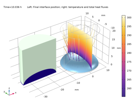
In the Title text area, type Left: Final interface position; right: temperature and total heat fluxes.
Slice 1
1
Right-click Sublimation Interface and choose Slice.
2
In the Settings window for Slice, locate the Expression section.
3
In the Expression text field, type T.
4
Locate the Plane Data section. In the Planes text field, type 1.
5
Locate the Coloring and Style section. From the Color table list, choose HeatCameraLight.
Isosurface 1
1
In the Model Builder window, right-click Sublimation Interface and choose Isosurface.
2
In the Settings window for Isosurface, locate the Expression section.
3
In the Expression text field, type Zg.
4
Locate the Levels section. From the Entry method list, choose Levels.
5
In the Levels text field, type Z0-Zi.
6
Locate the Coloring and Style section. From the Color table list, choose JupiterAuroraBorealis.
7
Clear the Color legend check box.
8
In the Sublimation Interface toolbar, click  Plot.
Streamline 1
1
Right-click Sublimation Interface and choose Streamline.
2
In the Settings window for Streamline, click Replace Expression in the upper-right corner of the Expression section. From the menu, choose Component 1 (comp1)>Heat Transfer in Porous Media>Domain fluxes>ht.tfluxx,...,ht.tfluxz - Total heat flux (spatial and material frames).
3
Locate the Streamline Positioning section. From the Positioning list, choose Magnitude controlled.
4
Locate the Coloring and Style section. Find the Line style subsection. From the Type list, choose Tube.
Color Expression 1
1
Right-click Streamline 1 and choose Color Expression.
2
In the Settings window for Color Expression, locate the Expression section.
3
In the Expression text field, type T.
4
Locate the Coloring and Style section. Clear the Color legend check box.
5
From the Color table list, choose HeatCameraLight.
Line 1
1
In the Model Builder window, right-click Sublimation Interface and choose Line.
2
In the Settings window for Line, locate the Expression section.
3
In the Expression text field, type 1.
4
Locate the Coloring and Style section. From the Coloring list, choose Uniform.
5
From the Color list, choose Gray.
6
In the Sublimation Interface toolbar, click  Plot.
Volume 1
1
Right-click Sublimation Interface and choose Volume.
2
In the Settings window for Volume, locate the Data section.
3
From the Dataset list, choose Study 1/Solution 1 (sol1).
4
Locate the Expression section. In the Expression text field, type dom==1||dom==3||dom==5.
5
Locate the Coloring and Style section. From the Color table list, choose AuroraBorealis.
6
Clear the Color legend check box.
Translation 1
1
Right-click Volume 1 and choose Translation.
2
In the Settings window for Translation, locate the Translation section.
3
In the x text field, type -2.5*R0.
4
In the y text field, type 0.
5
In the z text field, type 0.
6
Clear the Apply to dataset edges check box.
7
In the Sublimation Interface toolbar, click  Plot.
8
Click the  Zoom Extents button in the Graphics toolbar.
Temperature history
Plot the temperature variation during the primary drying at seven locations equally spread along the vial.
1
In the Home toolbar, click  Add Plot Group and choose 1D Plot Group.
2
In the Settings window for 1D Plot Group, type Temperature history in the Label text field.
3
Locate the Data section. From the Dataset list, choose None.
4
Click to expand the Title section. From the Title type list, choose Manual.
5
In the Title text area, type Temperature history at seven different heights at the center of the vial.
6
Locate the Plot Settings section. Select the x-axis label check box.
7
8
Select the y-axis label check box.
9
10
Locate the Legend section. From the Position list, choose Upper left.
Point Graph 1
1
Right-click Temperature history and choose Point Graph.
2
In the Settings window for Point Graph, locate the Data section.
3
From the Dataset list, choose Cut Point 3D 1.
4
Locate the y-Axis Data section. In the Expression text field, type T.
5
In the Temperature history toolbar, click  Plot.
6
Click to expand the Quality section. Click to expand the Coloring and Style section. In the Width text field, type 2.
7
Click to expand the Legends section. Select the Show legends check box.
8
From the Legends list, choose Evaluated.
9
In the Legend text field, type z/Z0=eval(z/Z0).
Ice mass
Then, plot the ice mass decreasing during the primary drying.
1
In the Home toolbar, click  Add Plot Group and choose 1D Plot Group.
2
In the Settings window for 1D Plot Group, type Ice mass in the Label text field.
3
Locate the Title section. From the Title type list, choose Manual.
4
In the Title text area, type Ice mass relative to initial amount.
5
Locate the Plot Settings section. Select the x-axis label check box.
6
7
Select the y-axis label check box.
8
9
Locate the Legend section. Clear the Show legends check box.
Global 1
1
Right-click Ice mass and choose Global.
2
In the Settings window for Global, locate the y-Axis Data section.
3
4
In the Ice mass toolbar, click  Plot.
5
Click to expand the Coloring and Style section. In the Width text field, type 2.
Initial Ice Mass
Finally, check the mass conservation: the difference between the initial and the final ice mass should be equal to the amount of vapor that has left the vial.
1
In the Results toolbar, click  Global Evaluation.
2
In the Settings window for Global Evaluation, type Initial Ice Mass in the Label text field.
3
Locate the Expressions section. In the table, enter the following settings:
4
Locate the Data Series Operation section. From the Transformation list, choose Maximum.
5
Click  Evaluate.
Final Ice Mass
1
Right-click Initial Ice Mass and choose Duplicate.
2
In the Settings window for Global Evaluation, type Final Ice Mass in the Label text field.
3
Locate the Data Series Operation section. From the Transformation list, choose Minimum.
4
Click  Evaluate.
Vapor Flux
1
In the Results toolbar, click  More Derived Values and choose Integration>Surface Integration.
2
In the Settings window for Surface Integration, type Vapor Flux in the Label text field.
3
4
Locate the Expressions section. In the table, enter the following settings:
5
Locate the Integration Settings section. Select the Integration order check box.
6
Locate the Data Series Operation section. From the Transformation list, choose Integral.
7
Click  Evaluate.