|
|
|
|
1
|
|
2
|
|
3
|
Click Add.
|
|
4
|
Click
|
|
5
|
|
6
|
Click
|
|
1
|
|
2
|
|
3
|
|
4
|
Browse to the model’s Application Libraries folder and double-click the file cooling_solidification_metal_parameters.txt.
|
|
1
|
|
2
|
|
3
|
|
4
|
|
1
|
|
2
|
|
3
|
|
4
|
|
5
|
|
6
|
|
7
|
|
1
|
|
2
|
|
3
|
|
1
|
|
2
|
|
3
|
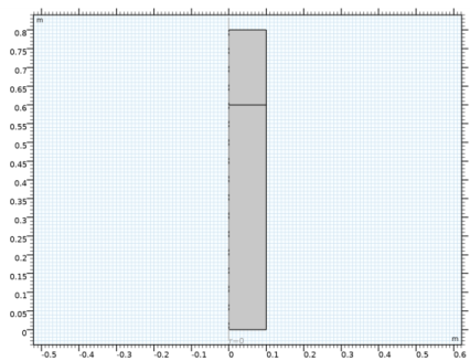
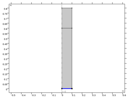
Click in the Graphics window and then press Ctrl+A to select both domains.
|
|
4
|
|
1
|
In the Model Builder window, under Component 1 (comp1)>Heat Transfer in Fluids (ht) click Initial Values 1.
|
|
2
|
|
3
|
|
1
|
|
2
|
|
3
|
Specify the u vector as
|
|
1
|
|
2
|
|
3
|
|
4
|
|
5
|
|
6
|
|
7
|
|
1
|
|
3
|
|
4
|
|
1
|
|
3
|
|
4
|
|
5
|
|
6
|
|
1
|
|
3
|
|
4
|
|
5
|
|
6
|
|
1
|
|
3
|
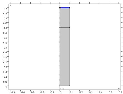
In the Settings window for Surface-to-Ambient Radiation, locate the Surface-to-Ambient Radiation section.
|
|
4
|
|
5
|
|
1
|
|
1
|
|
2
|
|
3
|
|
1
|
|
2
|
|
3
|
|
1
|
|
2
|
|
3
|
|
4
|
Click
|
|
6
|
Click to expand the Adaptation and Error Estimates section. From the Adaptation and error estimates list, choose Adaptation and error estimates.
|
|
7
|
|
8
|
|
1
|
|
2
|
In the Settings window for 2D Plot Group, type Solid and Liquid Phases (Adaptive Mesh) in the Label text field.
|
|
1
|
|
2
|
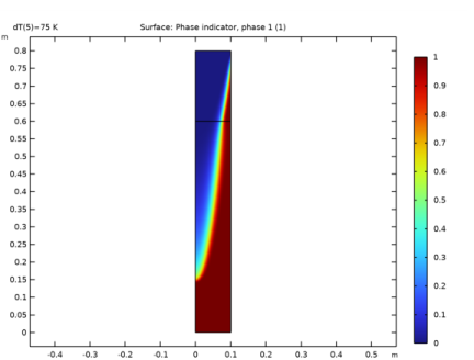
In the Settings window for Surface, click Replace Expression in the upper-right corner of the Expression section. From the menu, choose Component 1 (comp1)>Heat Transfer in Fluids>Phase change>ht.theta1 - Phase indicator, phase 1.
|
|
3
|
|
1
|
|
2
|
|
3
|
|
4
|
|
5
|
|
1
|
|
2
|
|
3
|
|
1
|
|
2
|
|
3
|
Find the Initial values of variables solved for subsection. From the Settings list, choose User controlled.
|
|
4
|
|
5
|
|
6
|
|
7
|
|
8
|
|
9
|
Click to expand the Mesh Selection section. Locate the Study Extensions section. Select the Auxiliary sweep check box.
|
|
10
|
Click
|
|
1
|
|
2
|
|
3
|
|
4
|
|
5
|
|
1
|
|
2
|
|
3
|
|
1
|
|
2
|
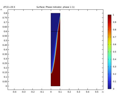
In the Settings window for Surface, click Replace Expression in the upper-right corner of the Expression section. From the menu, choose Component 1 (comp1)>Heat Transfer in Fluids>Phase change>ht.theta1 - Phase indicator, phase 1.
|
|
3
|
|
1
|
|
2
|
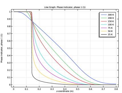
In the Settings window for 1D Plot Group, type Phase Indicator at Symmetry Axis in the Label text field.
|
|
1
|
|
3
|
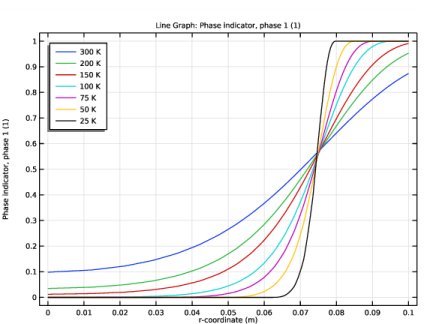
In the Settings window for Line Graph, click Replace Expression in the upper-right corner of the y-Axis Data section. From the menu, choose Component 1 (comp1)>Heat Transfer in Fluids>Phase change>ht.theta1 - Phase indicator, phase 1.
|
|
4
|
|
5
|
|
6
|
|
1
|
|
2
|
|
3
|
|
4
|
|
5
|
|
1
|
|
2
|
In the Settings window for 1D Plot Group, type Phase Indicator through Radius in the Label text field.
|
|
1
|
In the Model Builder window, expand the Phase Indicator through Radius node, then click Line Graph 1.
|
|
2
|
|
3
|
|
5
|
|
6
|
|
1
|
|
2
|
|
3
|
|
5
|
|
1
|
|
2
|
|
3
|
|
4
|