|
|
|
|
1
|
|
2
|
|
3
|
Click Add.
|
|
4
|
Click
|
|
5
|
|
6
|
Click
|
|
1
|
|
2
|
|
1
|
|
2
|
|
4
|
|
1
|
|
2
|
|
4
|
|
1
|
|
2
|
|
3
|
|
4
|
|
5
|
|
6
|
|
7
|
|
1
|
|
1
|
|
3
|
|
4
|
|
5
|
|
6
|
Click OK.
|
|
1
|
|
2
|
|
3
|
|
4
|
|
5
|
|
6
|
|
7
|
|
1
|
|
1
|
|
3
|
|
4
|
|
1
|
In the Model Builder window, under Component 1 (comp1)>Multiphysics click Nonisothermal Flow 1 (nitf1).
|
|
2
|
|
3
|
|
1
|
|
2
|
|
3
|
|
1
|
In the Model Builder window, under Component 1 (comp1)>Heat Transfer in Fluids (ht) click Initial Values 1.
|
|
2
|
|
3
|
|
1
|
|
1
|
|
3
|
|
4
|
|
1
|
|
3
|
|
4
|
|
5
|
|
6
|
|
7
|
|
8
|
|
9
|
|
10
|
|
1
|
|
3
|
|
4
|
|
5
|
|
6
|
|
1
|
|
2
|
|
3
|
|
4
|
|
1
|
|
2
|
|
3
|
|
4
|
|
5
|
|
1
|
|
2
|
|
3
|
|
4
|
|
5
|
|
6
|
|
1
|
|
2
|
|
1
|
|
2
|
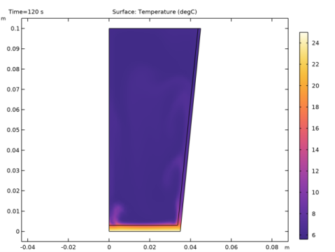
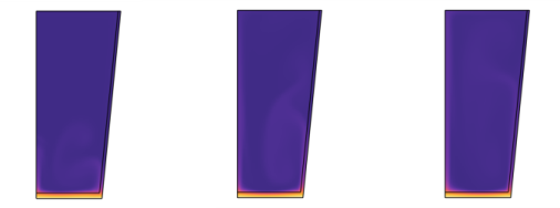
In the Settings window for Surface, click Replace Expression in the upper-right corner of the Expression section. From the menu, choose Component 1 (comp1)>Heat Transfer in Fluids>Temperature>T - Temperature - K.
|
|
3
|
|
4
|
|
5
|
|
6
|
|
1
|
|
2
|
|
3
|
|
4
|
|
1
|
|
2
|
|
1
|
|
2
|
|
3
|
|
4
|
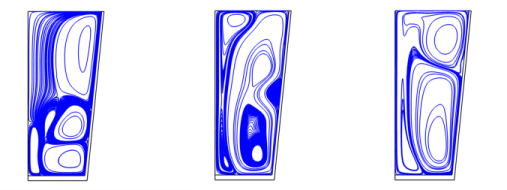
Locate the Coloring and Style section. Find the Point style subsection. From the Color list, choose Blue.
|
|
1
|
|
2
|
|
3
|
|
4
|
|
1
|
|
3
|
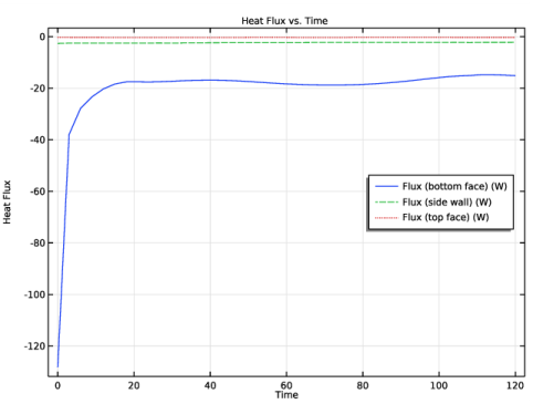
In the Settings window for Line Integration, click Replace Expression in the upper-right corner of the Expressions section. From the menu, choose Component 1 (comp1)>Heat Transfer in Fluids>Boundary fluxes>ht.ntflux - Normal total heat flux - W/m².
|
|
4
|
Replace the variable description by Flux (bottom face).
|
|
5
|
Click
|
|
1
|
|
3
|
In the Settings window for Line Integration, click Replace Expression in the upper-right corner of the Expressions section. From the menu, choose Component 1 (comp1)>Heat Transfer in Fluids>Boundary fluxes>ht.ntflux - Normal total heat flux - W/m².
|
|
4
|
Replace the variable description by Flux (side wall).
|
|
5
|
Click
|
|
1
|
|
3
|
In the Settings window for Line Integration, click Replace Expression in the upper-right corner of the Expressions section. From the menu, choose Component 1 (comp1)>Heat Transfer in Fluids>Boundary fluxes>ht.ntflux - Normal total heat flux - W/m².
|
|
4
|
Replace the variable description by Flux (top face).
|
|
5
|
Click
|
|
1
|
|
2
|
|
3
|
|
4
|
|
5
|
|
7
|
|
8
|
In the associated text field, type Heat Flux.
|
|
9
|
|
10
|
|
11
|
|
1
|
|
2
|
|
3
|
|
4
|
|
1
|
|
2
|
|
3
|
|
4
|
Locate the Coloring and Style section. Find the Line style subsection. From the Line list, choose Dashed.
|
|
5
|
|
6
|
|
1
|
|
2
|
|
3
|
|
1
|
|
2
|
|
3
|
|
4
|
Locate the Coloring and Style section. Find the Line style subsection. From the Line list, choose Dotted.
|
|
5
|
|
6
|