|
|
|


|
1
|
|
2
|
|
3
|
Click Add.
|
|
4
|
Click
|
|
5
|
|
6
|
Click
|
|
1
|
|
2
|
|
1
|
|
2
|
|
3
|
|
4
|
|
5
|
|
6
|
|
1
|
|
2
|
|
3
|
|
4
|
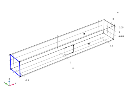
On the object blk1, select Boundary 3 only.
|
|
5
|
|
1
|
|
2
|
|
3
|
|
4
|
|
5
|
|
1
|
|
2
|
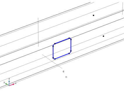
On the object r1, select Points 1–4 only.
|
|
3
|
|
4
|
|
1
|
|
2
|
|
3
|
|
4
|
|
1
|
|
2
|
|
3
|
|
4
|
|
5
|
|
1
|
|
2
|
|
4
|
|
5
|
|
1
|
|
1
|
|
2
|
|
3
|
|
1
|
|
1
|
In the Model Builder window, expand the Linear Elastic Material 2 node, then click Shell Local System 1.
|
|
2
|
|
3
|
|
1
|
|
3
|
In the Settings window for Prescribed Displacement/Rotation, locate the Prescribed Displacement section.
|
|
4
|
|
5
|
|
6
|
|
1
|
|
1
|
|
2
|
|
3
|
Specify the M vector as
|
|
4
|
|
1
|
|
2
|
|
3
|
Specify the M vector as
|
|
4
|
|
1
|
|
2
|
|
3
|
Specify the M vector as
|
|
4
|
|
1
|
|
2
|
|
1
|
|
2
|
|
1
|
|
2
|
|
1
|
In the Model Builder window, under Global Definitions>Load and Constraint Groups click Load Group 1.
|
|
2
|
|
3
|
|
1
|
|
2
|
|
3
|
|
1
|
|
2
|
|
3
|
|
1
|
In the Model Builder window, under Component 1 (comp1) right-click Materials and choose Blank Material.
|
|
3
|
|
1
|
|
2
|
|
3
|
|
4
|
|
1
|
|
2
|
|
3
|
|
4
|
Click Add three times.
|
|
6
|
|
7
|
|
8
|
|
1
|
|
3
|
In the Settings window for Point Evaluation, click Replace Expression in the upper-right corner of the Expressions section. From the menu, choose Component 1 (comp1)>Shell>Strain>Strain tensor (local)>shell.el11 - Strain tensor (local), 11 component.
|
|
4
|
Locate the Expressions section. In the table, enter the following settings:
|
|
5
|
Find the Parameters subsection. In the table, enter the following settings:
|
|
6
|
Click
|
|
1
|
|
2
|
In the Settings window for Point Evaluation, click Replace Expression in the upper-right corner of the Expressions section. From the menu, choose Component 1 (comp1)>Shell>Strain>Strain tensor (local)>shell.el22 - Strain tensor (local), 22 component.
|
|
3
|
Locate the Expressions section. In the table, enter the following settings:
|
|
4
|
Click
|
|
1
|
In the Model Builder window, under Results>Derived Values right-click Point Evaluation 1 and choose Duplicate.
|
|
3
|
|
5
|
Click
|
|
1
|
|
2
|
|
3
|
|
4
|
Click
|
|
5
|
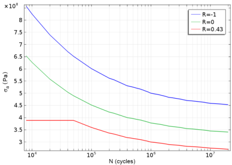
Browse to the model’s Application Libraries folder and double-click the file frame_with_cutout_SN_curve.txt.
|
|
6
|
Click
|
|
1
|
|
2
|
|
3
|
|
4
|
Click
|
|
5
|
Browse to the model’s Application Libraries folder and double-click the file frame_with_cutout_load.txt.
|
|
6
|
|
7
|
Click
|
|
8
|
Find the Functions subsection. In the table, enter the following settings:
|
|
1
|
|
2
|
|
3
|
|
4
|
Find the Physics interfaces in study subsection. In the table, clear the Solve check box for Study: Generalized Loads.
|
|
5
|
|
6
|
|
1
|
|
3
|
|
4
|
|
5
|
|
6
|
|
7
|
Locate the Cycle Counting Parameters section. Find the Discretization subsection. In the Nr text field, type 20.
|
|
8
|
|
9
|
|
10
|
|
11
|
Click
|
|
1
|
|
2
|
|
3
|
Find the Physics interfaces in study subsection. In the table, clear the Solve check box for Shell (shell).
|
|
4
|
Find the Studies subsection. In the Select Study tree, select Preset Studies for Selected Physics Interfaces>Fatigue.
|
|
5
|
|
6
|
|
1
|
|
2
|
Find the Values of variables not solved for subsection. From the Settings list, choose User controlled.
|
|
3
|
|
4
|
|
5
|
|
6
|
|
7
|
|
1
|
In the Model Builder window, under Results, Ctrl-click to select Fatigue Usage Factor (ftg), Stress Cycle Distribution (ftg), and Fatigue Usage Distribution (ftg).
|
|
2
|
Right-click and choose Group.
|
|
1
|
|
2
|
|
3
|
|
4
|
In the Expression text field, type
|
|
5
|
|
6
|
Select the Description check box.
|
|
7
|
In the associated text field, type Cutout angle.
|
|
8
|
|
1
|
|
2
|
In the Settings window for 1D Plot Group, type Fatigue Usage Factor Outside (ftg) in the Label text field.
|
|
1
|
|
2
|
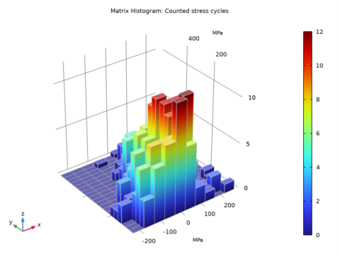
In the Settings window for 2D Plot Group, type Stress Cycle Distribution Outside (ftg) in the Label text field.
|
|
1
|
In the Model Builder window, expand the Stress Cycle Distribution Outside (ftg) node, then click Matrix Histogram 1.
|
|
2
|
|
3
|
|
4
|
|
5
|
|
1
|
|
2
|
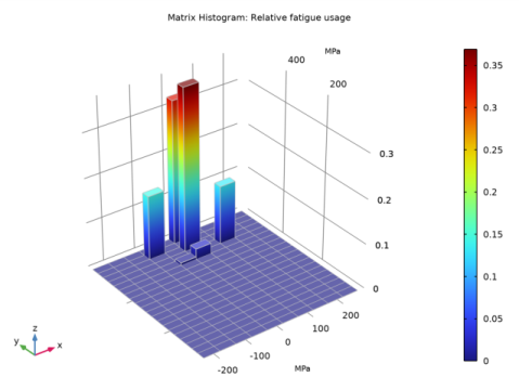
In the Settings window for 2D Plot Group, type Fatigue Usage Distribution Outside (ftg) in the Label text field.
|
|
1
|
In the Model Builder window, expand the Fatigue Usage Distribution Outside (ftg) node, then click Matrix Histogram 1.
|
|
2
|
|
3
|
|
4
|
|
5
|
|
1
|
|
2
|
|
3
|
|
4
|
Find the Physics interfaces in study subsection. In the table, clear the Solve check boxes for Study: Generalized Loads and Study: Fatigue Outside.
|
|
5
|
|
6
|
|
1
|
|
3
|
|
4
|
|
5
|
|
6
|
|
7
|
Locate the Cycle Counting Parameters section. Find the Discretization subsection. In the Nr text field, type 20.
|
|
8
|
|
9
|
|
10
|
|
11
|
Click Add three times.
|
|
1
|
|
2
|
|
3
|
Find the Physics interfaces in study subsection. In the table, clear the Solve check boxes for Shell (shell) and Fatigue Outside (ftg).
|
|
4
|
Find the Studies subsection. In the Select Study tree, select Preset Studies for Selected Physics Interfaces>Fatigue.
|
|
5
|
|
6
|
|
1
|
|
2
|
Find the Values of variables not solved for subsection. From the Settings list, choose User controlled.
|
|
3
|
|
4
|
|
5
|
|
6
|
|
7
|
|
1
|
In the Model Builder window, under Results, Ctrl-click to select Fatigue Usage Factor (ftg2), Stress Cycle Distribution (ftg2), and Fatigue Usage Distribution (ftg2).
|
|
2
|
Right-click and choose Group.
|
|
1
|
|
2
|
In the Settings window for 1D Plot Group, type Fatigue Usage Factor Inside (ftg2) in the Label text field.
|
|
1
|
In the Model Builder window, expand the Fatigue Usage Factor Inside (ftg2) node, then click Line Graph 1.
|
|
2
|
|
3
|
|
4
|
In the Expression text field, type
|
|
5
|
|
6
|
Select the Description check box.
|
|
7
|
In the associated text field, type Cutout angle.
|
|
8
|
|
1
|
|
2
|
In the Settings window for 2D Plot Group, type Stress Cycle Distribution Inside (ftg2) in the Label text field.
|
|
1
|
In the Model Builder window, expand the Stress Cycle Distribution Inside (ftg2) node, then click Matrix Histogram 1.
|
|
2
|
|
3
|
|
4
|
|
5
|
|
1
|
|
2
|
In the Settings window for 2D Plot Group, type Fatigue Usage Distribution Inside (ftg2) in the Label text field.
|
|
1
|
In the Model Builder window, expand the Fatigue Usage Distribution Inside (ftg2) node, then click Matrix Histogram 1.
|
|
2
|
|
3
|
|
4
|
|
5
|