You are viewing the documentation for an older COMSOL version. The latest version is available here.
PDF

Electrochemical Machining of a Microbore
Introduction
Electrochemical Machining (ECM) is based on the anodic dissolution of a metallic work piece. ECM has the advantages of a relatively low operating temperature (<80 °C) in combination with a process basically free of mechanical forces.
Microbores are used in various precision applications, such as hydraulic systems and fuel injectors. For a direct-injection fuel system the shape of the injection hole is of paramount importance for the combustion process.
This example models a primary current distribution and the resulting shape evolution of a bore during electrochemical machining.
Model Definition
The model geometry is shown in Figure 1. The electrolyte is fed into the cell from the top boundary at high velocity and exits through the bore at the bottommost boundary. A potential difference of 20 V is applied between the anode work piece and cathode tool, causing gas evolution on the cathode and metal dissolution or removal on the anode. An insulating layer is placed on top of the anode.
Figure 1: Model geometry. The geometry is symmetrical around the axis r=0.
Since only small potential gradients are expected in the electrodes due to the high metal conductivities, the electrode domains are not included in the model. The insulating layer is electrochemically inert and is hence not included either. The only modeled domain is the electrolyte.
Due to the high velocity of the flowing electrolyte, causing turbulent mixing, the electrolyte conductivity is assumed to be constant (7 S/m). In addition, the activation potentials of the electrode reactions are assumed to negligible so that a primary current distribution can be used to model the cell. The cathode is grounded and the anode is set to 20 V. The same equilibrium potential is used for both electrodes.
The anode electrode reaction gives rise to a boundary geometry deformation velocity vn (m/s) in the normal direction defined as
where M (kg/mol) is the molar mass and ρ (kg/m3) the density of the dissolving metal, n the number of electrons involved in the dissolution reaction, F (C/mol) Faraday’s constant, and iloc (A/m2) is the local current density of the electrode reaction. For a primary current distribution iloc can be calculated as
where il (A/m2) is the electrolyte current density vector and n the boundary normal.
veff is the effective stoichiometric coefficient for the metal in the anode electrode reaction. From experiments it has been seen that no metal dissolution occurs for current densities below 10 A/cm2. veff is therefore defined as:
Note that a current efficiency lower than unity is an indication of multiple competing electrode reactions being present, for instance oxygen evolution. A more detailed model would consider a secondary current distribution including multiple, competing, electrode reactions.
All other boundaries but the anode are set to zero geometrical deformation in the normal direction.
The electrochemical machining of the bore is simulated in a time-dependent study for 1 s.
Results and Discussion
Figure 2 shows the electrolyte potential distribution in the cell and the corresponding current density streamlines at = 1 s. The current is concentrated around the top of the workpiece.
Figure 2: Electrolyte potential and electrolyte current density streamlines at t = 1 s.
Figure 3 shows the profile of the workpiece at t = 0, 0.5, and 1 s. Most of the material removal occurs in the region located closest to the cathode tool, which is located outside the upper-left corner of the figure, but the material removal also reaches a less pronounced local maximum toward the right. This latter local maximum is an effect of the insulating layer.
Figure 4 shows a revolved plot of the current density at the workpiece surface at t = 1 s. For the lower parts of the bore the current density does not exceed the threshold current density for material removal (10 A/cm2).
Figure 3: Geometry deformation of the bore mouth at t = 0, 0.5 and 1 s.
Figure 4: Anode current density and geometry shape at t = 1 s.
Notes About the COMSOL Implementation
A small rectangular seed deformation along the anode at z=0, extending into/below the insulating layer is introduced in the initial geometry (see Figure 3, t = 0 graph). The reason for this is to avoid singularities in the contact point between the electrolyte and the insulating boundary, and to enforce a zero vertical deformation along the insulator/anode contact line (the dotted line in Figure 1).
The default Nondeforming Boundary node is modified to use a Zero normal displacement type of boundary condition for the geometry deformation. This ensures that all corners are fixed in the geometry.
Reference
1. M. Hackert-Oschätzchen, M. Kowalick, G. Meichsner, and A. Schubert, “Multiphysics Simulation of the Electrochemical Finishing of Micro Bores,” Proceedings of the 2012 COMSOL Conference in Milan, 2012.
Application Library path: Electrodeposition_Module/Tutorials/ecm_microbore
Modeling Instructions
From the File menu, choose New.
New
In the New window, click  Model Wizard.
Model Wizard
1
In the Model Wizard window, click  2D Axisymmetric.
2
In the Select Physics tree, select Electrochemistry>Electrodeposition, Deformed Geometry>Electrodeposition, Primary.
3
Click Add.
4
Click  Study.
5
In the Select Study tree, select General Studies>Time Dependent.
6
Global Definitions
Load the model parameters from a text file.
Parameters 1
1
In the Model Builder window, under Global Definitions click Parameters 1.
2
In the Settings window for Parameters, locate the Parameters section.
3
Click  Load from File.
4
Geometry 1
Set the default length unit of the model to millimeters.
1
In the Model Builder window, under Component 1 (comp1) click Geometry 1.
2
In the Settings window for Geometry, locate the Units section.
3
From the Length unit list, choose mm.
Rectangle 1 (r1)
Now draw the geometry as a set of rectangles and polygons.
1
In the Geometry toolbar, click  Rectangle.
2
In the Settings window for Rectangle, locate the Size and Shape section.
3
In the Width text field, type 3.
4
In the Height text field, type 3.
5
Locate the Position section. In the z text field, type -1.
Polygon 1 (pol1)
1
In the Geometry toolbar, click  Polygon.
2
In the Settings window for Polygon, locate the Coordinates section.
3
Polygon 2 (pol2)
1
In the Geometry toolbar, click  Polygon.
2
In the Settings window for Polygon, locate the Coordinates section.
3
Polygon 3 (pol3)
1
In the Geometry toolbar, click  Polygon.
2
In the Settings window for Polygon, locate the Coordinates section.
3
Difference 1 (dif1)
1
In the Geometry toolbar, click  Booleans and Partitions and choose Difference.
2
3
In the Settings window for Difference, locate the Difference section.
4
Find the Objects to subtract subsection. Click to select the  Activate Selection toggle button.
5
Select the objects pol1, pol2, and pol3 only.
6
Click  Build Selected.
Rectangle 2 (r2)
1
In the Geometry toolbar, click  Rectangle.
2
In the Settings window for Rectangle, locate the Size and Shape section.
3
In the Width text field, type 0.25+s_seed*3-a2.
4
In the Height text field, type s_seed.
5
Locate the Position section. In the r text field, type a2.
6
In the z text field, type -s_seed.
Union 1 (uni1)
1
In the Geometry toolbar, click  Booleans and Partitions and choose Union.
2
Click in the Graphics window and then press Ctrl+A to select both objects.
3
In the Settings window for Union, locate the Union section.
4
Clear the Keep interior boundaries check box.
5
Click the  Zoom Extents button in the Graphics toolbar.
6
Click  Build All Objects.
Your finished geometry should now look like this:
Definitions
Now define some selections of the geometry. They will be used later when setting up the physics.
Anode
1
In the Definitions toolbar, click  Explicit.
2
In the Settings window for Explicit, locate the Input Entities section.
3
From the Geometric entity level list, choose Boundary.
4
Click  Paste Selection.
5
In the Paste Selection dialog box, type 6-7, 10 in the Selection text field.
6
7
Right-click Explicit 1 and choose Rename.
8
In the Rename Explicit dialog box, type Anode in the New label text field.
9
Cathode
1
In the Definitions toolbar, click  Explicit.
2
In the Settings window for Explicit, locate the Input Entities section.
3
From the Geometric entity level list, choose Boundary.
4
Click  Paste Selection.
5
In the Paste Selection dialog box, type 3, 4 in the Selection text field.
6
7
Right-click Explicit 2 and choose Rename.
8
In the Rename Explicit dialog box, type Cathode in the New label text field.
9
Cathode tip
1
In the Definitions toolbar, click  Explicit.
2
In the Settings window for Explicit, locate the Input Entities section.
3
From the Geometric entity level list, choose Boundary.
4
5
Right-click Explicit 3 and choose Rename.
6
In the Rename Explicit dialog box, type Cathode tip in the New label text field.
7
Add a step function that will be used later when defining the 10 A/cm2 threshold current density for material removal.
Step 1 (step1)
In the Definitions toolbar, click  More Functions and choose Step.
Primary Current Distribution (cd)
Electrolyte 1
Now set up the physics. Start with the electrolyte.
1
In the Settings window for Electrolyte, locate the Electrolyte section.
2
From the σl list, choose User defined. In the associated text field, type sigma.
Electrode Surface 1
Use an Electrode Surface to describe the anode. Add a Dissolving-Depositing species to define the deformation velocity.
1
In the Model Builder window, right-click Primary Current Distribution (cd) and choose Electrode Surface.
2
In the Settings window for Electrode Surface, locate the Boundary Selection section.
3
From the Selection list, choose Anode.
4
Locate the Electrode Phase Potential Condition section. In the φs,ext text field, type E_cell.
5
Click to expand the Dissolving-Depositing Species section. Click  Add.
6
7
Clear the Solve for surface concentration variables check box.
Electrode Reaction 1
1
In the Model Builder window, click Electrode Reaction 1.
2
In the Settings window for Electrode Reaction, locate the Stoichiometric Coefficients section.
3
In the n text field, type n.
The stoichiometric coefficient will determine the direction and velocity of the geometry deformation. Use the step function you defined before to set the velocity to zero below a certain threshold current density.
4
In the Stoichiometric coefficients for dissolving-depositing species: table, enter the following settings:
Electrode Surface 2
Use a second Electrode Surface feature to define the cathode.
1
In the Physics toolbar, click  Boundaries and choose Electrode Surface.
2
In the Settings window for Electrode Surface, locate the Boundary Selection section.
3
From the Selection list, choose Cathode.
Multiphysics
Nondeforming Boundary 1 (ndbdg1)
The following applies a stronger constraint (than the default condition) for the planar nondepositing walls in order to enforce a zero boundary movement in the normal direction.
1
In the Model Builder window, under Component 1 (comp1)>Multiphysics click Nondeforming Boundary 1 (ndbdg1).
2
In the Settings window for Nondeforming Boundary, locate the Nondeforming Boundary section.
3
From the Boundary condition list, choose Zero normal displacement.
Deforming Electrode Surface 1 (desdg1)
Two of the electrode boundaries are not deforming. Deselect the corresponding boundaries from the Deforming Electrode Surface node.
1
In the Model Builder window, click Deforming Electrode Surface 1 (desdg1).
2
In the Settings window for Deforming Electrode Surface, locate the Boundary Selection section.
3
4
Click  Remove from Selection.
5
Mesh 1
Create a user-defined mesh with higher resolution on the electrodes.
1
In the Model Builder window, under Component 1 (comp1) click Mesh 1.
2
In the Settings window for Mesh, locate the Sequence Type section.
3
From the list, choose User-controlled mesh.
Size
1
In the Model Builder window, under Component 1 (comp1)>Mesh 1 click Size.
2
In the Settings window for Size, locate the Element Size section.
3
From the Predefined list, choose Finer.
4
Click to expand the Element Size Parameters section. In the Resolution of narrow regions text field, type 3.
Size 1
1
In the Model Builder window, right-click Free Triangular 1 and choose Size.
2
In the Settings window for Size, locate the Geometric Entity Selection section.
3
From the Geometric entity level list, choose Boundary.
4
From the Selection list, choose Anode.
5
Locate the Element Size section. Click the Custom button.
6
Locate the Element Size Parameters section. Select the Maximum element size check box.
7
Size 2
1
Right-click Free Triangular 1 and choose Size.
2
In the Settings window for Size, locate the Geometric Entity Selection section.
3
From the Geometric entity level list, choose Boundary.
4
From the Selection list, choose Cathode tip.
5
Locate the Element Size section. Click the Custom button.
6
Locate the Element Size Parameters section. Select the Maximum element size check box.
7
8
In the Model Builder window, right-click Mesh 1 and choose Build All.
Study 1
Step 1: Time Dependent
Enable automatic remeshing. Then solve the model.
1
In the Model Builder window, under Study 1 click Step 1: Time Dependent.
2
In the Settings window for Time Dependent, click to expand the Study Extensions section.
3
Select the Automatic remeshing check box.
4
In the Home toolbar, click  Compute.
Results
Electrolyte Potential (cd)
The following will reproduce the plots from the Results and Discussion section. Start by disabling the arrow plot and instead adding streamlines to the default electrolyte potential plot.
Streamline 1
1
In the Model Builder window, expand the Electrolyte Potential (cd) node, then click Streamline 1.
2
In the Settings window for Streamline, locate the Streamline Positioning section.
3
From the Positioning list, choose Magnitude controlled.
4
In the Density text field, type 8.
5
In the Electrolyte Potential (cd) toolbar, click  Plot.
6
Click the  Zoom Extents button in the Graphics toolbar.
Bore Shape
Create line plots of the shape of the bore as follows:
1
In the Home toolbar, click  Add Plot Group and choose 1D Plot Group.
2
In the Settings window for 1D Plot Group, type Bore Shape in the Label text field.
Line Graph 1
1
Right-click Bore Shape and choose Line Graph.
2
In the Settings window for Line Graph, locate the Data section.
3
From the Dataset list, choose Study 1/Remeshed Solution 1 (sol2).
4
From the Time selection list, choose First.
5
Locate the Selection section. From the Selection list, choose Anode.
6
Locate the y-Axis Data section. In the Expression text field, type z.
7
Locate the x-Axis Data section. From the Parameter list, choose Expression.
8
In the Expression text field, type r.
9
Click to expand the Legends section. Select the Show legends check box.
10
In the Bore Shape toolbar, click  Plot.
Line Graph 2
1
Right-click Line Graph 1 and choose Duplicate.
2
In the Settings window for Line Graph, locate the Data section.
3
From the Time selection list, choose Interpolated.
4
In the Times (s) text field, type 0.5.
5
In the Bore Shape toolbar, click  Plot.
Line Graph 3
1
Right-click Line Graph 2 and choose Duplicate.
2
In the Settings window for Line Graph, locate the Data section.
3
In the Times (s) text field, type 1.
Line Graph 4
1
Right-click Line Graph 3 and choose Duplicate.
2
3
In the Settings window for Line Graph, click to expand the Coloring and Style section.
4
From the Color list, choose Black.
5
Locate the Legends section. Clear the Show legends check box.
Bore Shape
1
In the Model Builder window, click Bore Shape.
2
In the Settings window for 1D Plot Group, click to expand the Title section.
3
From the Title type list, choose Manual.
4
In the Title text area, type Bore shape for t=0, 0.5 and 1 s.
5
Locate the Axis section. Select the Manual axis limits check box.
6
In the x minimum text field, type 0.
7
In the x maximum text field, type 0.3.
8
In the y minimum text field, type -0.2.
9
In the y maximum text field, type 0.01.
10
Locate the Legend section. From the Position list, choose Lower right.
11
In the Bore Shape toolbar, click  Plot.
Follow these steps to create a revolved dataset for the anode surface. Then plot the current density on this surface in 3D.
Study 1/Remeshed Solution 1 (3) (sol2)
1
In the Model Builder window, expand the Results>Datasets node.
2
Right-click Results>Datasets>Study 1/Remeshed Solution 1 (sol2) and choose Duplicate.
Selection
1
In the Results toolbar, click  Attributes and choose Selection.
2
In the Settings window for Selection, locate the Geometric Entity Selection section.
3
From the Geometric entity level list, choose Boundary.
4
From the Selection list, choose Anode.
Revolution 2D 2
1
In the Results toolbar, click  More Datasets and choose Revolution 2D.
2
In the Settings window for Revolution 2D, locate the Data section.
3
From the Dataset list, choose Study 1/Remeshed Solution 1 (3) (sol2).
Current Density on the Bore Surface
1
In the Results toolbar, click  3D Plot Group.
2
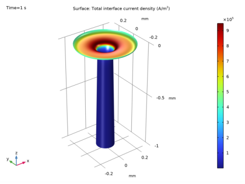
In the Settings window for 3D Plot Group, type Current Density on the Bore Surface in the Label text field.
3
Locate the Data section. From the Dataset list, choose Revolution 2D 2.
4
Locate the Plot Settings section. Clear the Plot dataset edges check box.
Surface 1
1
Right-click Current Density on the Bore Surface and choose Surface.
2
In the Settings window for Surface, click Replace Expression in the upper-right corner of the Expression section. From the menu, choose Component 1 (comp1)>Primary Current Distribution>Electrode kinetics>cd.itot - Total interface current density - A/m².
3
In the Current Density on the Bore Surface toolbar, click  Plot.
4
Click the  Zoom Extents button in the Graphics toolbar.
Finally, create an animation of the electromachining process in the following way.
Animation 1
1
In the Results toolbar, click  Animation and choose File.
2
In the Settings window for Animation, locate the Target section.
3
From the Target list, choose Player.
4
Locate the Scene section. From the Subject list, choose Current Density on the Bore Surface.
5
Locate the Animation Editing section. From the Time selection list, choose Interpolated.
6
Click  Range.
7
In the Range dialog box, type 0 in the Start text field.
8
In the Step text field, type 0.1.
9
In the Stop text field, type 1.
10
Click Replace.
11
Click the  Play button in the Graphics toolbar.