You are viewing the documentation for an older COMSOL version. The latest version is available here.
PDF

Copper Deposition in a Through-Hole Via
Introduction
Copper electrodeposition in a Through-Hole (TH) via is prevalent in electronic industry, particularly for the Printed Circuit Boards (PCBs). This model demonstrates the “butterfly” filling mechanism of the TH via during copper electrodeposition. Due to the presence of halide-suppressor additives in the electrolyte, electrodeposition occurs selectively at the center of the via, thus avoiding the formation of electrolyte enclosures. The example is based on a scientific paper (Ref. 1).
The purpose of the model is to demonstrate the use of deforming geometries for plating processes and the use of the Adsorbing-Desorbing Species functionlaity to model the influence of a suppressor on the plating result.
Model Definition
The model is defined by the material balances for the involved species (copper, Cu2+,chloride, Cl- and suppressor additive polyether, P) in the electrolyte solution and the adsorbed species (chloride, Cl and suppressor additive polyether, P) on the electrode surface, as well as an electrolyte charge balance assuming the presence of a supporting electrolyte.
The model geometry is shown in Figure 1. A 2D axi-symmetric space dimension is considered in the model. The upper horizontal boundary represents the anode and the cathode is placed at the bottom. The rightmost and leftmost vertical walls correspond to insulation (axial symmetry). The bottommost horizontal boundary corresponds to symmetry.
Figure 1: Model domain with boundaries corresponding to the anode, cathode, and symmetry walls.
The flux for each of the species in the electrolyte is given by the Nernst–Planck equation
where Ni denotes the transport vector (mol/(m2·s)), ci the concentration in the electrolyte (mol/m3), zi the charge for the ionic species, ui the mobility of the charged species (m2/(s·J·mole)), F Faraday’s constant (As/mole), and the potential in the electrolyte (V). The material balances are expressed through
one for each species, that is i = 1, 2 and 3.
The electrolyte charge transport is solved assuming a supporting electrolyte charge conservation model according to
At the cathode surface, copper electrodeposition reaction occurs according to
The boundary condition for the cathode is given by the Butler-Volmer equation for copper deposition. This gives the following relation for the local current density as a function of potential and copper concentration
where η denotes the overpotential defined as
where denotes the electronic potential of the respective electrode. The equilibrium potentials for the copper reduction reaction is calculated using the Nernst Equation
The exchange current density, , is defined is defined in terms of surface coverage of the suppressor additive polyether, P, and the cupric ion concentration according to
(1)
where is the unsuppressed reference exchange current density, is the suppressed reference exchange current density and is the surface coverage of the suppressor additive polyether, P.
The flux condition for the copper ions at the cathode boundary is defined as
where n denotes the normal vector to the boundary.
For the chloride ions, flux condition is defined as
For the suppressor additive polyether, P, flux condition is defined as
Using the Electrode Surface boundary node, with an added Dissolving-Depositing species, the ion fluxes and the boundary mesh velocity are based on the reaction currents, the number of electrons, and the specified stoichiometric coefficients of the electrode reactions. The sign of the stoichiometric coefficient for a species depends on whether the species is getting oxidized (positive) or reduced (negative) in the reaction. The stoichiometric coefficient is for the copper ions in the electrolyte, whereas that for the copper atoms in the electrode is .
Using the Electrode Surface boundary node, with an added Adsorbing-Desorbing species, surface coverage is evaluated according to
where and are adsorption kinetics, and are deactivation kinetics for chloride and suppressor, respectively, and deposition velocity, v (m/s), is calculated according to
where M is the mean molar mass (63.55 g/mol) and ρ is the density (8960 kg/m3) of the nickel atoms and n is number of participating electrons.
At the anode surface, the electrolyte potential is set to 0 and concentration of all involved species is set to their initial concentrations.
All other boundaries are insulating.
The initial conditions set the composition of the electrolyte according to
You set up the above equations using the Tertiary Current Distribution, Nernst–Planck Equations interface. The Deformed Geometry node keeps track of the deformation of the mesh.
Results and Discussion
Figure 2 shows the surface plot for concentration distribution of chloride ions along with contour plot and the displacement of the cathode surface after 14.5 minutes of operation. The figure clearly shows that copper electrodeposition occurs selectively at the center of the TH and grows radially inwards, leading to sidewall impingement at the TH via center and resulting in “butterfly” filling of copper in the TH via. The selective copper electrodeposition, avoiding the formation of undesirable electrolyte entrapment, is attributed to chloride-polyether additives adsorption-desorption at the cathode surface. The chloride ion concentration depletion can also be seen in Figure 2 towards the center of the TH via.
Figure 2: Chloride ion concentration (mol/m3) along with contour plot and electrode displacement in the cell after 14.5 minutes of operation.
Figure 3 shows the thickness of the deposition from the center along the vertical cathodic surface of the TH via. The lines reveal the development of the nonuniform deposition which is found to be more towards the center of via when compared to the mouth of the via.
Figure 3: Thickness of the deposition from the center along the vertical cathode boundary of TH via.
Figure 4 shows the surface coverage of chloride ions along the vertical cathodic surface of the TH via. The lines reveal that adsorption of additive (chloride) begins at the mouth of the TH via and then gradually covers the entire surface of the TH via. The surface coverage of additives is found to be the lowest at the center of the TH via leading the highest copper electrodepsosition in that region.
Figure 4: Surface coverage of chloride ions from the center along the vertical cathode boundary of TH via.
Reference
1. T. M. Braun, D. Josell, J. John and T. P. Moffat, “Simulation of Copper Electrodeposition in Though-Hole Vias,” Journal of The Electrochemical Society, vol. 167, 013510, 2020.
Application Library path: Electrodeposition_Module/Tutorials/cu_deposition_suppressor
Modeling Instructions
From the File menu, choose New.
New
In the New window, click  Model Wizard.
Model Wizard
1
In the Model Wizard window, click  2D Axisymmetric.
2
In the Select Physics tree, select Electrochemistry>Electrodeposition, Deformed Geometry>Electrodeposition, Tertiary with Supporting Electrolyte.
3
Click Add.
4
In the Number of species text field, type 3.
5
In the Concentrations table, enter the following settings:
6
Click  Study.
7
In the Select Study tree, select Preset Studies for Selected Physics Interfaces>Time Dependent with Initialization.
8
Geometry 1
Draw the geometry by making a union of two rectangles. Round off the corner of the hole using a fillet.
Rectangle 1 (r1)
1
In the Geometry toolbar, click  Rectangle.
2
In the Settings window for Rectangle, locate the Size and Shape section.
3
In the Width text field, type 15e-6.
4
In the Height text field, type 25e-6.
5
Locate the Position section. In the z text field, type 20e-6.
Rectangle 2 (r2)
1
In the Geometry toolbar, click  Rectangle.
2
In the Settings window for Rectangle, locate the Size and Shape section.
3
In the Width text field, type 5e-6.
4
In the Height text field, type 20e-6.
5
Click  Build Selected.
6
Click the  Zoom Extents button in the Graphics toolbar.
Union 1 (uni1)
1
In the Geometry toolbar, click  Booleans and Partitions and choose Union.
2
In the Settings window for Union, locate the Union section.
3
Clear the Keep interior boundaries check box.
4
Click in the Graphics window and then press Ctrl+A to select both objects.
Fillet 1 (fil1)
1
In the Geometry toolbar, click  Fillet.
2
On the object uni1, select Point 5 only.
3
In the Settings window for Fillet, locate the Radius section.
4
In the Radius text field, type 1e-6.
Form Union (fin)
1
In the Model Builder window, click Form Union (fin).
2
In the Settings window for Form Union/Assembly, click  Build Selected.
Global Definitions
Parameters 1
1
In the Model Builder window, under Global Definitions click Parameters 1.
2
In the Settings window for Parameters, locate the Parameters section.
3
Click  Load from File.
4
Definitions
Load the model variables from a text file.
Variables 1
1
In the Home toolbar, click  Variables and choose Local Variables.
2
In the Settings window for Variables, locate the Variables section.
3
Click  Load from File.
4
Tertiary Current Distribution, Nernst-Planck (tcd)
Now set up the electrochemical model, starting with the Electrolyte node.
Electrolyte 1
1
In the Model Builder window, under Component 1 (comp1)>Tertiary Current Distribution, Nernst-Planck (tcd) click Electrolyte 1.
2
In the Settings window for Electrolyte, locate the Diffusion section.
3
In the DcCu text field, type D_Cu.
4
In the DcCl text field, type D_Cl.
5
In the DcP text field, type D_P.
6
Locate the Migration in Electric Field section. In the zcCu text field, type z_Cu.
7
In the zcCl text field, type z_Cl.
8
Locate the Electrolyte Current Conduction section. From the σl list, choose User defined. In the associated text field, type sigmal.
Electrode Surface 1
1
In the Physics toolbar, click  Boundaries and choose Electrode Surface.
2
Create a selection of the boundaries to facilitate choosing this electrode surface later on when post processing the problem.
3
In the Settings window for Electrode Surface, locate the Boundary Selection section.
4
Click  Create Selection.
5
In the Create Selection dialog box, type Cathode in the Selection name text field.
6
7
In the Settings window for Electrode Surface, click to expand the Dissolving-Depositing Species section.
8
9
The dissolving-depositing species Cu contributes to the deposition velocity.
10
Click to expand the Adsorbing-Desorbing Species section. In the Γs text field, type Gamma_Cl.
11
12
13
14
Locate the Electrode Phase Potential Condition section. In the φs,ext text field, type phis_cathode.
Electrode Reaction 1
1
In the Model Builder window, click Electrode Reaction 1.
2
In the Settings window for Electrode Reaction, locate the Stoichiometric Coefficients section.
3
In the n text field, type 2.
4
In the νcCu text field, type -1.
5
In the Stoichiometric coefficients for dissolving-depositing species: table, enter the following settings:
6
Locate the Equilibrium Potential section. In the Eeq,ref(T) text field, type Erev.
7
Locate the Electrode Kinetics section. In the i0,ref(T) text field, type i0ref.
8
In the αa text field, type alpha_a.
Electrode Surface 1
Next, set the flux for species cCl and cP and reaction rates for adsorbing-desorbing species Cl and P using the Non-Faradaic Reactions node.
1
In the Model Builder window, click Electrode Surface 1.
Non-Faradaic Reactions 1
1
In the Physics toolbar, click  Attributes and choose Non-Faradaic Reactions.
2
In the Settings window for Non-Faradaic Reactions, locate the Reaction Rate section.
3
Select the Species cCl check box.
4
In the R0,cCl text field, type R_Cl.
5
Select the Species cP check box.
6
In the R0,cP text field, type R_P.
7
In the Reaction rate for adsorbing-desorbing species table, enter the following settings:
Electrolyte Potential 1
Next, set the electrolyte potential at the top boundary.
1
In the Physics toolbar, click  Boundaries and choose Electrolyte Potential.
2
Concentration 1
Next, also set the concentration of all spcies at the top boundary.
1
In the Physics toolbar, click  Boundaries and choose Concentration.
2
3
In the Settings window for Concentration, locate the Concentration section.
4
Select the Species cCu check box.
5
In the c0,cCu text field, type c0_Cu.
6
Select the Species cCl check box.
7
In the c0,cCl text field, type c0_Cl.
8
Select the Species cP check box.
9
In the c0,cP text field, type c0_P.
Symmetry 1
Finally, define the symmetry boundaries.
1
In the Physics toolbar, click  Boundaries and choose Symmetry.
2
Initial Values 1
1
In the Model Builder window, click Initial Values 1.
2
In the Settings window for Initial Values, locate the Initial Values section.
3
In the cCu text field, type c0_Cu.
4
In the cCl text field, type c0_Cl.
5
In the cP text field, type c0_P.
Multiphysics
Nondeforming Boundary 1 (ndbdg1)
1
In the Model Builder window, under Component 1 (comp1)>Multiphysics click Nondeforming Boundary 1 (ndbdg1).
2
In the Settings window for Nondeforming Boundary, locate the Nondeforming Boundary section.
3
From the Boundary condition list, choose Zero normal displacement.
Global Definitions
Default Model Inputs
Set up the temperature value to be used in the entire model.
1
In the Model Builder window, under Global Definitions click Default Model Inputs.
2
In the Settings window for Default Model Inputs, locate the Browse Model Inputs section.
3
In the tree, select General>Temperature (K) - minput.T.
4
Find the Expression for remaining selection subsection. In the Temperature text field, type T0.
Mesh 1
Define a physics-controlled extra fine mesh.
1
In the Model Builder window, under Component 1 (comp1) click Mesh 1.
2
In the Settings window for Mesh, locate the Physics-Controlled Mesh section.
3
From the Element size list, choose Extra fine.
4
Click  Build All.
Study 1
Select only Tertiary Current Distribution, Nernst Planck (tcd) interface to be solved for in the first study step.
Step 1: Current Distribution Initialization
1
In the Model Builder window, under Study 1 click Step 1: Current Distribution Initialization.
2
In the Settings window for Current Distribution Initialization, locate the Physics and Variables Selection section.
3
In the table, clear the Solve for check box for Deformed geometry (Component 1).
4
In the table, clear the Solve for check boxes for Nondeforming Boundary 1 (ndbdg1) and Deforming Electrode Surface 1 (desdg1).
Step 2: Time Dependent
1
In the Model Builder window, click Step 2: Time Dependent.
2
In the Settings window for Time Dependent, locate the Study Settings section.
3
From the Time unit list, choose min.
4
In the Output times text field, type range(0,0.5,14.5).
5
In the Home toolbar, click  Compute.
Results
Several plots are added by default. Now, to reproduce the plots from the Results and Discussion section, follow the below steps.
Mirror 3D 1
1
In the Results toolbar, click  More Datasets and choose Mirror 3D.
2
In the Settings window for Mirror 3D, locate the Plane Data section.
3
From the Plane list, choose XY-planes.
Concentration, Cl, 3D (tcd)
Next, plot the chloride concentration using the mirror dataset.
1
In the Model Builder window, under Results click Concentration, Cl, 3D (tcd).
2
In the Settings window for 3D Plot Group, locate the Data section.
3
From the Dataset list, choose Mirror 3D 1.
Contour 1
Right-click Concentration, Cl, 3D (tcd) and choose Contour.
Contour 1
1
In the Model Builder window, expand the Results>Concentration, Cl, 3D (tcd) node, then click Contour 1.
2
In the Settings window for Contour, click Replace Expression in the upper-right corner of the Expression section. From the menu, choose Component 1 (comp1)>Tertiary Current Distribution, Nernst-Planck>Species cCl>cCl - Concentration - mol/m³.
3
Locate the Coloring and Style section. From the Coloring list, choose Uniform.
4
From the Color list, choose Black.
5
Clear the Color legend check box.
6
In the Concentration, Cl, 3D (tcd) toolbar, click  Plot.
The plot should look like Figure 2.
Deposition thickness
Next, plot the deposition thickness along the vertical side of through-hole via.
1
In the Home toolbar, click  Add Plot Group and choose 1D Plot Group.
2
In the Settings window for 1D Plot Group, type Deposition thickness in the Label text field.
3
Click to expand the Title section. From the Title type list, choose Label.
Line Graph 1
1
In the Deposition thickness toolbar, click  Line Graph.
2
3
In the Settings window for Line Graph, locate the y-Axis Data section.
4
In the Expression text field, type tcd.sbtot.
5
From the Unit list, choose µm.
6
Locate the x-Axis Data section. From the Parameter list, choose Expression.
7
In the Expression text field, type z.
8
From the Unit list, choose µm.
9
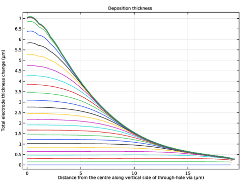
Select the Description check box.
10
In the associated text field, type Distance from the centre along vertical side of through-hole via.
11
In the Deposition thickness toolbar, click  Plot.
The plot should look like Figure 3.
Deposition thickness
Next, plot the surface coverage of chloride.
Surface coverage, Cl (tcd)
1
In the Model Builder window, right-click Deposition thickness and choose Duplicate.
2
In the Model Builder window, click Deposition thickness 1.
3
In the Settings window for 1D Plot Group, type Surface coverage, Cl (tcd) in the Label text field.
Line Graph 1
1
In the Model Builder window, click Line Graph 1.
2
In the Settings window for Line Graph, locate the y-Axis Data section.
3
In the Expression text field, type tcd.theta_es1_Cl.
4
In the Surface coverage, Cl (tcd) toolbar, click  Plot.
The plot should look like Figure 4.