PDF

Thin Layer Chronoamperometry
Introduction
Chronoamperometry is a technique in electroanalysis in which current drawn at an electrode is measured after a rapid step in the applied voltage.
In a thin-layer cell, the anode and cathode are separated by a microscale distance. This means that chemical species transport across the cell is fast, so an analyte in the cell can be consumed exhaustively after only a few seconds. By integrating the current transient (chronoamperogram), the initial concentration of analyte can be determined.
If the kinetics of the electrochemical reaction are always fast, there is no need to resolve the current density as a function of applied potential. Instead, the concentration of the analyte can be assumed to be driven to zero at the working electrode surface. Under this approximation, only the chemical species transport needs to be resolved.
Model Definition
This model contains a single 1D domain of length L = 60 μm, which is the thickness of the thin layer. Transport in plane with the anode and cathode is ignored; only normal transport is considered, which is assumed to be uniform across the cell.
DOMAIN EQUATIONS
The transport of the analyte obeys the diffusion equation (Fick’s second law):
The solution is assumed to be static (“quiescent”) so there is no mass transport by convection. A supporting electrolyte is present in high concentration, so the electric field is also taken to be zero. We do not model the product species as its concentration does not influence the current density.
BOUNDARY EQUATIONS
A high overpotential is applied so that the analyte undergoes a very fast electrochemical reaction at the working electrode surface (x = 0). To model this, the analyte concentration here is rapidly stepped to zero. The facing surface (x = L), is impermeable to the analyte — no flux is passed. We assume the counterreaction of the electrochemical cell to either take place at a physically separate counter electrode or to involve a distinct chemical species, present in excess, which we ignore in this model.
TIME-DEPENDENT STUDY
The Einstein equation gives the time for the mean position of a diffusion layer to cross a distance L, as a function of the diffusion coefficient D:
In the thin layer, the Einstein time is 0.9 s. After a few Einstein times, the analyte reacts to near exhaustion, and so the duration of the simulation is set to 5 s.
Results and Discussion
The concentration profiles through time demonstrate the growth of the diffusion layer across the cell (Figure 1).
Figure 1: Concentration profiles of the analyte across the thickness of the cell, as the experiment proceeds (from upper left to lower right).
Once the diffusion layer encounters the outer boundary of the cell, the concentration here begins to diminish as the continuing electrochemical reaction exhausts the available analyte.
As the diffusion layer expands, the flux at the working electrode becomes smaller. Correspondingly the current also decreases (Figure 2).
Figure 2: Measured chronoamperogram for the thin-layer cell.
From transport theory, the chronoamperometric current for an infinite expanse of bulk solution falls off inversely proportionally to the square root of time, as given by the Cottrell equation, where i is the current density, n is the number of electrons transferred per molecule of analyte, c is the bulk concentration of analyte, and D is its diffusion coefficient:
Figure 3: Simulated chronoamperogram compared on a logarithmic scale to the Cottrell equation for chronoamperometry with unlimited available analyte. The deviation at long times is caused by the finite quantity of analyte the cell.
By comparing the simulated results with the Cottrell equation, plotted on a logarithmic scale (Figure 3), good agreement is observed until roughly = 1 s. At this time — which is approximately the Einstein time noted above — the diffusion layer encounters the wall of the cell.
After this point, the current diminishes more quickly due to the exhaustion of available electroactive material for reaction. Under these conditions, the Cottrell equation no longer applies — the simulated current deviates negatively.
By integrating the concentration across the cell, we can calculate the proportion of the initial amount of analyte that has been consumed (Figure 4). After 5 seconds, 99% of the analyte has undergone an electrochemical reaction.
Figure 4: Proportion of the initial quantity of analyte that is consumed through the experiment.
References
1. R.G. Compton and C.E. Banks, Understanding Voltammetry, 2nd ed., World Scientific Publishing Co. Pte. Ltd, London, 2011.
2. A.J. Bard and L.R. Faulkner, Electrochemical Methods, Fundamentals and Applications, 2nd ed., Wiley, Hoboken, 2001.
3. F.G. Cottrell, Zeitschrift für Physikalische Chemie, vol. 42, pp. 385–431, 1903.
Application Library path: Electrochemistry_Module/Electroanalysis/thin_layer_chronoamperometry
Modeling Instructions
From the File menu, choose New.
New
In the New window, click  Model Wizard.
Model Wizard
1
In the Model Wizard window, click  1D.
2
In the Select Physics tree, select Electrochemistry>Electroanalysis (tcd).
3
Click Add.
4
In the Number of species text field, type 1.
5
In the Concentrations table, enter the following settings:
6
Click  Study.
7
In the Select Study tree, select General Studies>Time Dependent.
8
Global Definitions
Add the model parameters from a text file.
Parameters 1
1
In the Model Builder window, under Global Definitions click Parameters 1.
2
In the Settings window for Parameters, locate the Parameters section.
3
Click  Load from File.
4
Geometry 1
Create the model geometry as a single interval.
Interval 1 (i1)
1
In the Model Builder window, under Component 1 (comp1) right-click Geometry 1 and choose Interval.
2
In the Settings window for Interval, locate the Interval section.
3
4
In the Home toolbar, click  Build All.
Definitions
Add a smoothed step function that will be used to step the concentration at the electrode from initial conditions to zero as a continuous function of time.
Step 1 (step1)
1
In the Home toolbar, click  Functions and choose Local>Step.
2
In the Settings window for Step, locate the Parameters section.
3
In the Location text field, type 0.5.
4
Click to expand the Smoothing section. In the Size of transition zone text field, type 1.
Variables 1
Add some variables that will be used during postprocessing for comparing the simulated current with the Cottrell equation.
1
In the Home toolbar, click  Variables and choose Local Variables.
2
In the Settings window for Variables, locate the Variables section.
3
Electroanalysis (tcd)
Electrolyte 1
Now start setting up the physics. Start with the domain settings for the diffusion coefficient and the initial concentration.
1
In the Model Builder window, under Component 1 (comp1)>Electroanalysis (tcd) click Electrolyte 1.
2
In the Settings window for Electrolyte, locate the Diffusion section.
3
In the Dc text field, type D.
Initial Values 1
1
In the Model Builder window, click Initial Values 1.
2
In the Settings window for Initial Values, locate the Initial Values section.
3
In the c text field, type c_bulk.
Concentration 1
Set up the Concentration condition on the boundary using the step function defined above.
1
In the Physics toolbar, click  Boundaries and choose Concentration.
2
3
In the Settings window for Concentration, locate the Concentration section.
4
Select the Species c check box.
5
In the c0,c text field, type c_bulk*(1-step1(t/t_rise)).
Mesh 1
Refine the default mesh.
Size
1
In the Model Builder window, under Component 1 (comp1) right-click Mesh 1 and choose Edit Physics-Induced Sequence.
2
In the Settings window for Size, locate the Element Size section.
3
From the Predefined list, choose Extra fine.
Size 1
1
In the Model Builder window, right-click Edge 1 and choose Size.
2
In the Settings window for Size, locate the Geometric Entity Selection section.
3
From the Geometric entity level list, choose Boundary.
4
5
Locate the Element Size section. Click the Custom button.
6
Locate the Element Size Parameters section. Select the Maximum element size check box.
7
Edge 1
1
Right-click Edge 1 and choose Build Selected.
Your finished mesh should now look like this:
Study 1
Step 1: Time Dependent
Your model is now ready for solving. Solve for a time range of 5 s.
1
In the Model Builder window, under Study 1 click Step 1: Time Dependent.
2
In the Settings window for Time Dependent, locate the Study Settings section.
3
In the Output times text field, type range(0,0.1,5).
4
In the Home toolbar, click  Compute.
Results
Concentration (tcd)
The first default plot group shows the concentration.
Create the chronoamperogram as follows:
1D Plot Group 2
In the Home toolbar, click  Add Plot Group and choose 1D Plot Group.
Point Graph 1
1
Right-click 1D Plot Group 2 and choose Point Graph.
2
3
In the Settings window for Point Graph, locate the y-Axis Data section.
4
In the Expression text field, type i_el.
Chronoamperogram
1
In the Model Builder window, under Results click 1D Plot Group 2.
2
In the Settings window for 1D Plot Group, type Chronoamperogram in the Label text field.
3
Locate the Axis section. Select the Manual axis limits check box.
4
In the x minimum text field, type 0.1.
5
In the x maximum text field, type 5.
6
In the y minimum text field, type 0.
7
In the y maximum text field, type 5e-6.
8
In the Chronoamperogram toolbar, click  Plot.
Now, duplicate the chronoamperogram and compare, in log scale, the simulated curve to the Cottrell equation.
Comparison to Cottrell equation
1
Right-click Chronoamperogram and choose Duplicate.
2
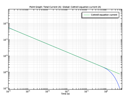
In the Settings window for 1D Plot Group, type Comparison to Cottrell equation in the Label text field.
Global 1
1
Right-click Comparison to Cottrell equation and choose Global.
2
In the Settings window for Global, locate the y-Axis Data section.
3
Comparison to Cottrell equation
1
In the Model Builder window, click Comparison to Cottrell equation.
2
In the Settings window for 1D Plot Group, locate the Axis section.
3
Clear the Manual axis limits check box.
4
Select the x-axis log scale check box.
5
Select the y-axis log scale check box.
6
In the Comparison to Cottrell equation toolbar, click  Plot.
7
Select the Manual axis limits check box.
8
In the x minimum text field, type 1e-5.
9
In the Comparison to Cottrell equation toolbar, click  Plot.
Finally, plot the extent of reaction by calculating the average amount of reacted concentration in a table, and then plotting the table data.
Line Average 1
1
In the Results toolbar, click  More Derived Values and choose Average>Line Average.
2
3
In the Settings window for Line Average, locate the Expressions section.
4
5
Clicknext to  Evaluate, then choose New Table.
Table
1
Go to the Table window.
2
Click Table Graph in the window toolbar.
Results
Extent of reaction
1
In the Model Builder window, under Results click 1D Plot Group 4.
2
In the Settings window for 1D Plot Group, type Extent of reaction in the Label text field.