PDF

Stress Corrosion
Introduction
Steel pipelines are often subjected to complex stress/strain conditions in oil and gas industry. In addition to stress from internal pressure, pipelines are subjected to significant longitudinal strain due to surrounding soil movement. As a result of the changed surface energies at the pipe surface, the resulting stresses may have an effect on the pipe corrosion rate. The intercoupled effects of elastic and plastic deformation on pipeline corrosion is demonstrated in this model example.
The elasto-plastic stress simulations are performed here using a small strain plasticity model and von-Mises yielding criterion. Iron dissolution (anodic) and hydrogen evolution (cathodic) are considered as electrochemical reactions, using kinetic expressions that account for the effect of elasto-plastic deformations.
The example is based on a paper by L. Y. Xu and Y. F. Cheng (Ref. 1). The model is built in two parts. In the first part, the stationary effect of the elasto-plastic stress on corrosion is investigated by varying the longitudinal strain using a parametric study. In the second part, a transient simulation is performed to investigate the intercoupled effects of a dissolving, and hence dynamically varying, corrosion defect depth on a pipe, subject to a constant strain.
Note: This model requires the Structural Mechanics, or the MEMS Module, with the addition of either the Nonlinear Structural Materials or the Geomechanics Module.
Model Definition
The model geometry is shown in Figure 1.
Figure 1: The model geometry consists of a pipeline with corrosion defect and surrounding soil domain.
The model geometry consists of high strength alloy steel pipeline and surrounding soil domain. The pipeline length is 2 m and wall thickness is 19.1 mm. The corrosion defect on the exterior side of the pipeline is elliptical in shape with a length of 200 mm and a depth of 11.46 mm. The electrolyte conductivity of soil domain in 0.096 S/m.
Elastoplastic Stress
An elastoplastic stress simulation is performed over pipeline domain using the small strain plasticity model. The user defined isotropic hardening model is used where the hardening function, σyhard, is defined as:
where σexp is the experimental stress-strain curve, εp is the plastic deformation, σe is the von Mises stress, E is the Young’s modulus (207·109 Pa), and σys is the yield strength of high strength alloy steel(806·106 Pa).
The experimental stress-strain curve used in the model is prescribed in terms of a piecewise cubic interpolation function and is taken from Ref. 2.
Electrochemical Reactions
The iron dissolution (anodic) and hydrogen evolution (cathodic) reactions are the two electrochemical reactions that occur at the corrosion defect surface of pipelines. The rest of pipeline surfaces are assumed to be electrochemically inactive.
An anodic Tafel expression is used to model the iron dissolution reaction, with a local anodic current density defined as
where i0,a is the exchange current density (2.353·103 A/m2), Aa is the Tafel slope (0.118 V) and the overpotential ηa for the anodic reaction is calculated from
The equilibrium potential for the anodic reaction is calculated from
where Eeq0,a is the standard equilibrium potential for the anodic reaction (0.859 V), ΔPm is the excess pressure to elastic deformation (2.687·108 Pa), Vm is the molar volume of steel (7.13·106 m3/mol), z is the charge number for steel (2), F is the Faraday’s constant, T is the absolute temperature (298.15 K), R is the ideal gas constant, νis an orientation dependent factor (0.45), α is a coefficient (1.67·1015 m-2) and N0 is the initial dislocation density (1·1012 m-2).
A cathodic Tafel expression is used to model the hydrogen evolution reaction, this sets the local cathodic current density to
where i0,c is the exchange current density, Ac is the Tafel slope (0.207 V) and the overpotential ηc (SI unit: V) for the cathodic reaction is calculated from
where Eeq0,c is the standard equilibrium potential for the cathodic reaction (0.644 V)
The exchange current density for the cathodic reaction is calculated from
where i0,c,ref is the reference exchange current density for the cathodic reaction in the absence of external stress/strain (1.457·102 A/m2).
Deformed geometry
In the second part of the model, dissolution of iron from the corrosion defect is modeled using deformed geometry. The dissolution of iron causes the electrode boundary to move, with a velocity in the normal direction, v (SI unit: m/s), according to
where ia (SI unit: A/m2) is the anodic current density, M is the molar mass (55.845 g/mol) and ρ the density (7870 kg/m3) of the iron.
Solve the model in a time-dependent study, simulating the corrosion for 20 years of exposure.
Results and Discussion
Figure 2 shows the electrolyte potential distribution (V) over the soil domain and the von Mises stress distribution (MPa) over the pipe domain, as indicated by the color bars for a prescribed displacement of 4 mm in the x direction. It can be seen that the local stresses are significantly higher near the corrosion defect than that at the rest of the pipeline. A nonuniform electrolyte potential distribution near the corrosion defect is also evident in Figure 2, as indicated by a semi-circular area.
Figure 2: The electrolyte potential distribution over the soil domain and the von Mises stress distribution over the pipeline domain for a prescribed displacement of 4 mm.
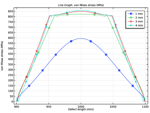
Figure 3 shows the von Mises stress distribution along the length of the corrosion defect for prescribed displacements of 1 mm, 2 mm, 3 mm, and 4 mm, respectively. The von Mises stress increases with an increase in the tensile strain and it is found to be maximum at the center of corrosion defect. For the tensile strain of 2 mm, 3 mm and 4 mm, it is observed that the local stress, particularly at the center of corrosion defect, exceeds the yield strength of high strength alloy steel (806·106 Pa). This results in the plastic deformation at the center of corrosion defect while deformation in the remaining area of corrosion defect remains in the elastic range. For the lower tensile strain of 1 mm, the entire corrosion defect is observed to be in the elastic deformation range.
Figure 3: The von Mises stress distribution along the length of the corrosion defect for prescribed displacements of 1 mm, 2 mm, 3 mm, and 4 mm.
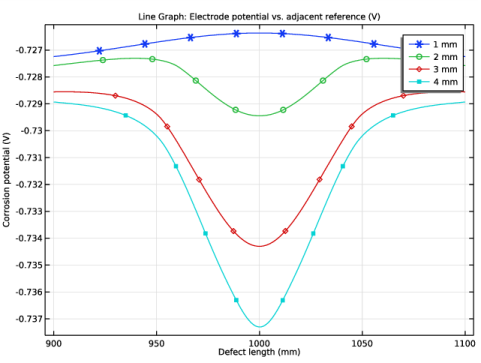
Figure 4 shows the corrosion potential distribution along the length of the corrosion defect for prescribed displacements of 1 mm, 2 mm, 3 mm, and 4 mm. For lower tensile strain of 1 mm, the variation in the corrosion potential is found to be uniform along the length of the corrosion defect. However, for higher tensile strains of 2 mm, 3 mm and 4 mm, the variation in the corrosion potential is nonuniform with the more negative corrosion potential at the center of the corrosion defect than that at both the sides of the corrosion defect.
Figure 4: The corrosion potential distribution along the length of the corrosion defect for prescribed displacements of 1 mm, 2 mm, 3 mm, and 4 mm.
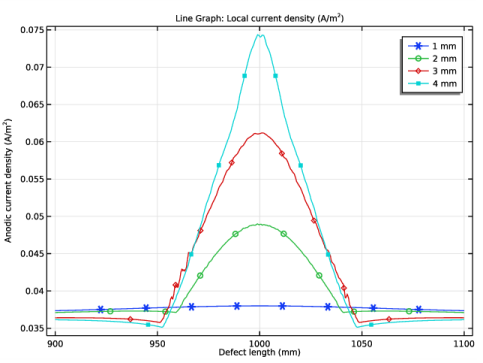
Figure 5 shows the anodic current density distribution along the length of corrosion defect for prescribed displacements of 1 mm, 2 mm, 3 mm, and 4 mm. For lower tensile strain of 1 mm, the variation in the anodic current density is found to be uniform along the length of the corrosion defect, similar to the corrosion potential behavior. However, for higher tensile strains of 2 mm, 3 mm and 4 mm, the variation in the anodic current density is significantly nonuniform, particularly at the center of the corrosion defect. It can be seen that the anodic current density increases significantly at the center of the corrosion defect whereas it decreases slightly at both the sides of the corrosion defect for higher tensile strains. The increase in the anodic current density for tensile strains of 2 mm, 3 mm and 4 mm is attributed to the plastic deformation observed at the center of the corrosion defect (see Figure 3).
Figure 5: The anodic current density distribution along the length of the corrosion defect for prescribed displacements of 1 mm, 2 mm, 3 mm, and 4 mm.
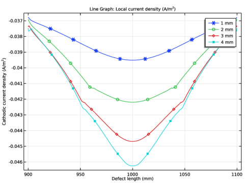
Figure 6 shows the cathodic current density distribution along the length of the corrosion defect for prescribed displacements of 1 mm, 2 mm, 3 mm, and 4 mm. It can be seen that the cathodic current density increases negatively with an increase in the tensile strain and it is found to be the most negative at the center of the corrosion defect. The nonuniformity in the cathodic current density is also found to increase with an increase in the tensile strain. Thus, the cathodic current density distribution is found to be the most nonuniform for a tensile strain of 4 mm.
Figure 6: The cathodic current density distribution along the length of the corrosion defect for prescribed displacements of 1 mm, 2 mm, 3 mm, and 4 mm.
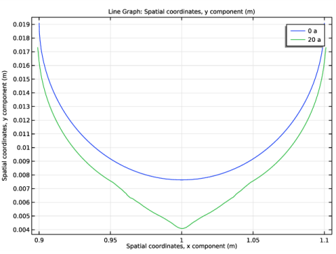
Figure 7 shows the corrosion defect profile at time t = 0 a and 20 a. It can be seen that after 20 years, the depth of the corrosion defect is increased particularly at the center of the corrosion defect.
Figure 7: The corrosion defect profile at time t = 0 a and 20 a.
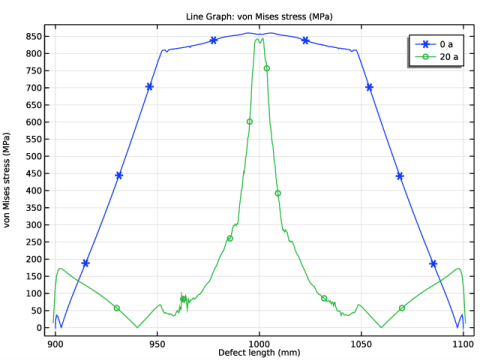
Figure 8 shows the von Mises stress distribution along the length of the corrosion defect at time t = 0 a and 20 a. It can be seen that after 20 years, the von Mises stress is higher at the center of the corrosion defect than that at both the sides of the corrosion defect.
Figure 8: The von Mises stress distribution along the length of the corrosion defect at time t = 0 a and 20 a.
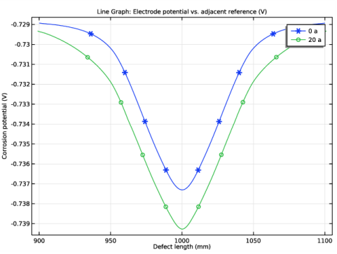
Figure 9 shows the corrosion potential distribution along the length of the corrosion defect at time t = 0 a and 20 a. It can be seen that after 20 years, the corrosion potential is more negative throughout the length of the corrosion defect.
Figure 9: The corrosion potential distribution along the length of the corrosion defect at time t = 0 a and 20 a.
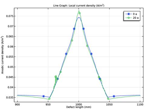
Figure 10 shows the anodic current density distribution along the length of corrosion defect at time t = 0 a and 20 a. It can be seen that after 20 years, the anodic current density is marginally higher at the center of the corrosion defect when compared with that at time t = 0 a.
Figure 10: The anodic current density distribution along the length of the corrosion defect at time t = 0 a and 20 a.
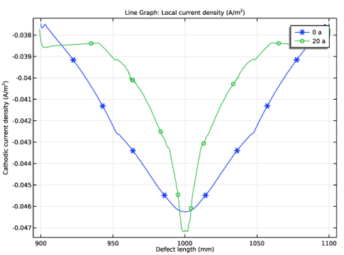
Figure 11 shows the cathodic current density distribution along the length of the corrosion defect at time t = 0 a and 20 a. It can be seen that after 20 years, the cathodic current density is more negative at the center of the corrosion defect than that at both the sides of the corrosion defect. The cathodic current density is also found to be marginally more negative at the center of the corrosion defect when compared with that at time t = 0 a.
Figure 11: The cathodic current density distribution along the length of the corrosion defect at time t = 0 a and 20 a.
Notes About the COMSOL Implementation
The model is implemented using the Solid Mechanics interface and the Secondary Current Distribution interface. In the first study, the Solid Mechanics model does not depend upon the results of the Secondary Current Distribution model, and we use a sequential solver set up with a Parametric Sweep to study the impact of elastoplastic deformations on electrochemical reactions. In the second part of the model, a transient analysis is performed using Deformed Geometry to analyze the effect of varying depth, due to dissolution, on stress as well as corrosion.
References
1. L. Y. Xu and Y. F. Cheng, “Development of a finite element model for simulation and prediction of mechanoelectrochemical effect of pipeline corrosion”, Corrosion Science, vol. 73, pp. 150–160, 2013.
2. L. Xu, “Assessment of corrosion defects on high-strength steel pipelines”, PhD thesis, Department of mechanical and manufacturing engineering, University of Calgary, Alberta, August 2013.
Application Library path: Corrosion_Module/General_Corrosion/stress_corrosion
Modeling Instructions
From the File menu, choose New.
New
In the New window, click  Model Wizard.
Model Wizard
1
In the Model Wizard window, click  2D.
2
In the Select Physics tree, select Structural Mechanics>Solid Mechanics (solid).
3
Click Add.
4
In the Select Physics tree, select Electrochemistry>Primary and Secondary Current Distribution>Secondary Current Distribution (cd).
5
Click Add.
6
Click  Study.
7
In the Select Study tree, select General Studies>Stationary.
8
Geometry 1
Draw the geometry for pipe with corrosion defect and surrounding soil domain.
Rectangle 1 (r1)
1
In the Geometry toolbar, click  Rectangle.
2
In the Settings window for Rectangle, locate the Size and Shape section.
3
In the Width text field, type 2.
4
In the Height text field, type 19.1[mm].
Ellipse 1 (e1)
1
In the Geometry toolbar, click  Ellipse.
2
In the Settings window for Ellipse, locate the Size and Shape section.
3
In the a-semiaxis text field, type 100[mm].
4
In the b-semiaxis text field, type 11.46[mm].
5
Locate the Position section. In the x text field, type 1.
6
In the y text field, type 19.1[mm].
Difference 1 (dif1)
1
In the Geometry toolbar, click  Booleans and Partitions and choose Difference.
2
3
In the Settings window for Difference, locate the Difference section.
4
Find the Objects to subtract subsection. Click to select the  Activate Selection toggle button.
5
Rectangle 2 (r2)
1
In the Geometry toolbar, click  Rectangle.
2
In the Settings window for Rectangle, locate the Size and Shape section.
3
In the Width text field, type 2.
4
Click  Build All Objects.
5
Click the  Zoom Extents button in the Graphics toolbar.
Your geometry should look like Figure 1.
Global Definitions
Parameters 1
Load the model parameters.
1
In the Model Builder window, under Global Definitions click Parameters 1.
2
In the Settings window for Parameters, locate the Parameters section.
3
Click  Load from File.
4
Definitions
Load the model variables.
Variables 1
1
In the Model Builder window, expand the Component 1 (comp1)>Definitions node.
2
Right-click Definitions and choose Variables.
3
In the Settings window for Variables, locate the Variables section.
4
Click  Load from File.
5
Interpolation 1 (int1)
Load the stress strain interpolation data from a text file.
1
In the Home toolbar, click  Functions and choose Local>Interpolation.
2
In the Settings window for Interpolation, locate the Definition section.
3
In the Function name text field, type stress_strain_curve.
4
Click  Load from File.
5
Browse to the model’s Application Libraries folder and double-click the file stress_corrosion_stress_strain_curve_interpolation.txt.
6
Locate the Interpolation and Extrapolation section. From the Interpolation list, choose Piecewise cubic.
7
Locate the Units section. In the Argument table, enter the following settings:
8
In the Function table, enter the following settings:
Solid Mechanics (solid)
Start setting up the physics. First, set the elastoplastic deformation at the Linear Elastic Material node by adding Plasticity node.
1
In the Model Builder window, under Component 1 (comp1) click Solid Mechanics (solid).
2
In the Settings window for Solid Mechanics, locate the Domain Selection section.
3
4
Click  Remove from Selection.
5
Linear Elastic Material 1
In the Model Builder window, under Component 1 (comp1)>Solid Mechanics (solid) click Linear Elastic Material 1.
Plasticity 1
1
In the Physics toolbar, click  Attributes and choose Plasticity.
2
In the Settings window for Plasticity, locate the Plasticity Model section.
3
Find the Isotropic hardening model subsection. From the list, choose Hardening function.
Materials
Now, add high-strength alloy steel material for pipe and set the values for initial yield stress, hardening function, Young’s modulus and Poisson’s ratio.
Add Material
1
In the Home toolbar, click  Add Material to open the Add Material window.
2
Go to the Add Material window.
3
In the tree, select Built-in>High-strength alloy steel.
4
Click Add to Component in the window toolbar.
5
In the Home toolbar, click  Add Material to close the Add Material window.
Materials
High-strength alloy steel (mat1)
1
In the Settings window for Material, locate the Geometric Entity Selection section.
2
3
Click  Remove from Selection.
4
In the table under Material Contents, set the value of Initial yield stress to 806e6 [Pa] and Hardening function to hardening. Also, change the value of Young’s modulus to 207e9 [Pa] and Poisson’s ratio to 0.33.
Solid Mechanics (solid)
Now, set the initial value for displacement field and then proceed to setting up boundary conditions for Solid Mechanics physics interface.
Initial Values 1
1
In the Model Builder window, under Component 1 (comp1)>Solid Mechanics (solid) click Initial Values 1.
2
In the Settings window for Initial Values, locate the Initial Values section.
3
Specify the u vector as
Fixed Constraint 1
1
In the Physics toolbar, click  Boundaries and choose Fixed Constraint.
2
Prescribed Displacement 1
1
In the Physics toolbar, click  Boundaries and choose Prescribed Displacement.
2
3
In the Settings window for Prescribed Displacement, locate the Prescribed Displacement section.
4
Select the Prescribed in x direction check box.
5
In the u0x text field, type disp.
Prescribed Displacement 2
1
In the Physics toolbar, click  Boundaries and choose Prescribed Displacement.
2
3
In the Settings window for Prescribed Displacement, locate the Prescribed Displacement section.
4
Select the Prescribed in x direction check box.
Fixed Constraint 2
1
In the Physics toolbar, click  Points and choose Fixed Constraint.
2
Secondary Current Distribution (cd)
Now, set up the physics for electrochemical reactions. First, set electrolyte conductivity, initial value for electrolyte potential and then set both anodic and cathodic reactions at the corrosion defect surface of pipe.
Electrolyte 1
1
In the Model Builder window, under Component 1 (comp1)>Secondary Current Distribution (cd) click Electrolyte 1.
2
In the Settings window for Electrolyte, locate the Electrolyte section.
3
From the σl list, choose User defined. In the associated text field, type sigmal.
Initial Values 1
1
In the Model Builder window, click Initial Values 1.
2
In the Settings window for Initial Values, locate the Initial Values section.
3
In the phil text field, type -(Eeq0a+Eeq0c)/2.
Electrode 1
1
In the Physics toolbar, click  Domains and choose Electrode.
2
3
In the Settings window for Electrode, locate the Electrode section.
4
From the σs list, choose User defined. In the associated text field, type sigmas.
Internal Electrode Surface 1
1
In the Physics toolbar, click  Boundaries and choose Internal Electrode Surface.
2
Electrode Reaction 1
1
In the Model Builder window, click Electrode Reaction 1.
2
In the Settings window for Electrode Reaction, locate the Equilibrium Potential section.
3
In the Eeq text field, type Eeqa.
4
Locate the Electrode Kinetics section. From the Kinetics expression type list, choose Anodic Tafel equation.
5
In the i0 text field, type i0a.
6
In the Aa text field, type ba.
Internal Electrode Surface 1
In the Model Builder window, click Internal Electrode Surface 1.
Electrode Reaction 2
1
In the Physics toolbar, click  Attributes and choose Electrode Reaction.
2
In the Settings window for Electrode Reaction, locate the Equilibrium Potential section.
3
In the Eeq text field, type Eeq0c.
4
Locate the Electrode Kinetics section. From the Kinetics expression type list, choose Cathodic Tafel equation.
5
In the i0 text field, type ic.
6
In the Ac text field, type bc.
Electric Ground 1
1
In the Physics toolbar, click  Boundaries and choose Electric Ground.
2
Mesh 1
Set the finer mesh near corrosion defect surface of pipe.
Free Triangular 1
In the Mesh toolbar, click  Free Triangular.
Size 1
1
Right-click Free Triangular 1 and choose Size.
2
In the Settings window for Size, locate the Geometric Entity Selection section.
3
From the Geometric entity level list, choose Domain.
4
5
Locate the Element Size section. Click the Custom button.
6
Locate the Element Size Parameters section. Select the Maximum element size check box.
7
Size 2
1
In the Model Builder window, right-click Free Triangular 1 and choose Size.
2
In the Settings window for Size, locate the Geometric Entity Selection section.
3
From the Geometric entity level list, choose Boundary.
4
5
Locate the Element Size section. Click the Custom button.
6
Locate the Element Size Parameters section. Select the Maximum element size check box.
7
8
Click  Build All.
Study: Stationary Parametric
Now, set the solver settings. Since solid mechanics physics is not dependent upon electrochemical reactions, we use a sequential solver setup with a parametric sweep.
1
In the Model Builder window, click Study 1.
2
In the Settings window for Study, type Study: Stationary Parametric in the Label text field.
Parametric Sweep
1
In the Study toolbar, click  Parametric Sweep.
2
In the Settings window for Parametric Sweep, locate the Study Settings section.
3
4
Step 1: Stationary
1
In the Model Builder window, click Step 1: Stationary.
2
In the Settings window for Stationary, locate the Physics and Variables Selection section.
3
In the table, clear the Solve for check box for Secondary Current Distribution (cd).
Stationary 2
1
In the Study toolbar, click  Study Steps and choose Stationary>Stationary.
2
In the Settings window for Stationary, locate the Physics and Variables Selection section.
3
In the table, clear the Solve for check box for Solid Mechanics (solid).
Solution 1 (sol1)
Lower the relative tolerance for Secondary Current Distribution study step.
1
In the Study toolbar, click  Show Default Solver.
2
In the Model Builder window, expand the Solution 1 (sol1) node, then click Stationary Solver 2.
3
In the Settings window for Stationary Solver, locate the General section.
4
In the Relative tolerance text field, type 0.00001.
Clear the Generate default plots check box. The model is now ready to be solved.
5
In the Model Builder window, click Study: Stationary Parametric.
6
In the Settings window for Study, locate the Study Settings section.
7
Clear the Generate default plots check box.
8
In the Study toolbar, click  Compute.
Results
Corrosion Potential and von Mises Stress
1
In the Home toolbar, click  Add Plot Group and choose 2D Plot Group.
2
In the Settings window for 2D Plot Group, type Corrosion Potential and von Mises Stress in the Label text field.
3
Locate the Data section. From the Dataset list, choose Study: Stationary Parametric/Parametric Solutions 1 (sol3).
Surface 1
1
In the Corrosion Potential and von Mises Stress toolbar, click  Surface.
2
In the Settings window for Surface, click Replace Expression in the upper-right corner of the Expression section. From the menu, choose Component 1 (comp1)>Solid Mechanics>Stress>solid.mises - von Mises stress - N/m².
3
Locate the Expression section. From the Unit list, choose MPa.
Corrosion Potential and von Mises Stress
In the Model Builder window, click Corrosion Potential and von Mises Stress.
Surface 2
1
In the Corrosion Potential and von Mises Stress toolbar, click  Surface.
2
In the Settings window for Surface, locate the Expression section.
3
In the Expression text field, type -phil.
4
Click to expand the Range section. Select the Manual color range check box.
5
In the Minimum text field, type -0.733.
6
In the Maximum text field, type -0.724.
7
Locate the Coloring and Style section. From the Color table transformation list, choose Reverse.
8
In the Corrosion Potential and von Mises Stress toolbar, click  Plot.
9
Click the  Zoom Extents button in the Graphics toolbar.
The plot should like Figure 2. One can zoom in a region close to corrosion defect using Zoom Box icon in the Graphics window.
von Mises Stress, Parametric
Plot von Mises stress along the corrosion defect for different values of prescribed displacements.
1
In the Home toolbar, click  Add Plot Group and choose 1D Plot Group.
2
In the Settings window for 1D Plot Group, type von Mises Stress, Parametric in the Label text field.
3
Locate the Data section. From the Dataset list, choose Study: Stationary Parametric/Parametric Solutions 1 (sol3).
4
Locate the Plot Settings section. Select the x-axis label check box.
5
Line Graph 1
1
In the von Mises Stress, Parametric toolbar, click  Line Graph.
2
3
In the Settings window for Line Graph, click Replace Expression in the upper-right corner of the y-Axis Data section. From the menu, choose Component 1 (comp1)>Solid Mechanics>Stress>solid.mises - von Mises stress - N/m².
4
Locate the y-Axis Data section. From the Unit list, choose MPa.
5
Locate the x-Axis Data section. From the Parameter list, choose Expression.
6
In the Expression text field, type x.
7
From the Unit list, choose mm.
8
Click to expand the Coloring and Style section. Find the Line markers subsection. From the Marker list, choose Cycle.
9
Click to expand the Legends section. Select the Show legends check box.
10
From the Legends list, choose Evaluated.
11
In the Legend text field, type eval(disp,mm) mm.
12
In the von Mises Stress, Parametric toolbar, click  Plot.
The plot should look like Figure 3.
von Mises Stress, Parametric
Now, plot corrosion potential along defect length for different prerscribed displacements.
Corrosion Potential, Parametric
1
In the Model Builder window, right-click von Mises Stress, Parametric and choose Duplicate.
2
In the Settings window for 1D Plot Group, type Corrosion Potential, Parametric in the Label text field.
3
Locate the Plot Settings section. Select the y-axis label check box.
4
In the associated text field, type Corrosion potential (V).
Line Graph 1
1
In the Model Builder window, expand the Corrosion Potential, Parametric node, then click Line Graph 1.
2
In the Settings window for Line Graph, click Replace Expression in the upper-right corner of the y-Axis Data section. From the menu, choose Component 1 (comp1)>Secondary Current Distribution>cd.Evsref - Electrode potential vs. adjacent reference - V.
3
In the Corrosion Potential, Parametric toolbar, click  Plot.
The plot should look like Figure 4.
Corrosion Potential, Parametric
Plot the anodic current density along the corrosion defect.
Anodic Current Density, Parametric
1
In the Model Builder window, right-click Corrosion Potential, Parametric and choose Duplicate.
2
In the Settings window for 1D Plot Group, type Anodic Current Density, Parametric in the Label text field.
3
Locate the Plot Settings section. In the y-axis label text field, type Anodic current density (A/m<sup>2</sup>).
Line Graph 1
1
In the Model Builder window, expand the Anodic Current Density, Parametric node, then click Line Graph 1.
2
In the Settings window for Line Graph, click Replace Expression in the upper-right corner of the y-Axis Data section. From the menu, choose Component 1 (comp1)>Secondary Current Distribution>Electrode kinetics>cd.iloc_er1 - Local current density - A/m².
3
In the Anodic Current Density, Parametric toolbar, click  Plot.
The plot should look like Figure 5.
Anodic Current Density, Parametric
Plot the cathodic current density along the corrosion defect.
Cathodic Current Density, Parametric
1
In the Model Builder window, right-click Anodic Current Density, Parametric and choose Duplicate.
2
In the Settings window for 1D Plot Group, type Cathodic Current Density, Parametric in the Label text field.
3
Locate the Plot Settings section. In the y-axis label text field, type Cathodic current density (A/m<sup>2</sup>).
Line Graph 1
1
In the Model Builder window, expand the Cathodic Current Density, Parametric node, then click Line Graph 1.
2
In the Settings window for Line Graph, click Replace Expression in the upper-right corner of the y-Axis Data section. From the menu, choose Component 1 (comp1)>Secondary Current Distribution>Electrode kinetics>cd.iloc_er2 - Local current density - A/m².
3
In the Cathodic Current Density, Parametric toolbar, click  Plot.
The plot should look like Figure 6.
Component 1 (comp1)
In the second part of the model, we add Deformed Geometry to investigate the impact of deformation due to dissolution on stress distribution and hence, subsequently on corrosion.
1
In the Definitions toolbar, click  Deformed Geometry and choose Domains>Deforming Domain.
Deformed Geometry
Deforming Domain 1
1
In the Settings window for Deforming Domain, locate the Domain Selection section.
2
From the Selection list, choose All domains.
3
Locate the Smoothing section. From the Mesh smoothing type list, choose Hyperelastic.
Secondary Current Distribution (cd)
Next, add Dissolving-Depositing Species to capture dissolution at the electrode surface.
Internal Electrode Surface 1
1
In the Model Builder window, under Component 1 (comp1)>Secondary Current Distribution (cd) click Internal Electrode Surface 1.
2
In the Settings window for Internal Electrode Surface, click to expand the Dissolving-Depositing Species section.
3
4
Electrode Reaction 1
1
In the Model Builder window, click Electrode Reaction 1.
2
In the Settings window for Electrode Reaction, locate the Stoichiometric Coefficients section.
3
In the Stoichiometric coefficients for dissolving-depositing species: table, enter the following settings:
Multiphysics
Next, set multiphysics features for deformed geometry.
Nondeforming Boundary 1 (ndbdg1)
1
In the Physics toolbar, click  Multiphysics Couplings and choose Boundary>Nondeforming Boundary.
2
In the Settings window for Nondeforming Boundary, locate the Boundary Selection section.
3
From the Selection list, choose All boundaries.
4
Locate the Nondeforming Boundary section. From the Boundary condition list, choose Zero normal displacement.
Deforming Electrode Surface 1 (desdg1)
1
In the Physics toolbar, click  Multiphysics Couplings and choose Boundary>Deforming Electrode Surface.
2
In the Settings window for Deforming Electrode Surface, locate the Boundary Selection section.
3
From the Selection list, choose All boundaries.
Study: Stationary Parametric
Before setting up transient study, disable appropriate nodes in the Stationary Parametric study for completeness.
Step 1: Stationary
1
In the Model Builder window, expand the Study: Stationary Parametric node, then click Step 1: Stationary.
2
In the Settings window for Stationary, locate the Physics and Variables Selection section.
3
4
Step 2: Stationary 2
1
In the Model Builder window, click Step 2: Stationary 2.
2
In the Settings window for Stationary, locate the Physics and Variables Selection section.
3
4
Root
Finally, add a new time dependent study to capture the deformation.
Add Study
1
In the Home toolbar, click  Add Study to open the Add Study window.
2
Go to the Add Study window.
3
Find the Studies subsection. In the Select Study tree, select General Studies>Time Dependent.
4
Click Add Study in the window toolbar.
5
In the Home toolbar, click  Add Study to close the Add Study window.
Study 2
Step 1: Time Dependent
1
In the Settings window for Time Dependent, locate the Study Settings section.
2
From the Time unit list, choose a.
3
In the Output times text field, type range(0,1,20).
4
Click to expand the Values of Dependent Variables section. Find the Initial values of variables solved for subsection. From the Settings list, choose User controlled.
5
From the Method list, choose Solution.
6
From the Study list, choose Study: Stationary Parametric, Stationary 2.
7
From the Solution list, choose Parametric Solutions 1 (sol3).
8
In the Model Builder window, click Study 2.
9
In the Settings window for Study, type Study: Transient, Deformed Geometry in the Label text field.
10
Locate the Study Settings section. Clear the Generate default plots check box.
Solution 8 (sol8)
1
In the Study toolbar, click  Show Default Solver.
2
In the Model Builder window, expand the Solution 8 (sol8) node.
3
In the Model Builder window, expand the Study: Transient, Deformed Geometry>Solver Configurations>Solution 8 (sol8)>Time-Dependent Solver 1 node, then click Fully Coupled 1.
4
In the Settings window for Fully Coupled, click to expand the Method and Termination section.
5
In the Maximum number of iterations text field, type 12.
6
In the Study toolbar, click  Compute.
Results
Corrosion Defect Profile
Now, plot the corrosion defect profile for the first and last time steps.
1
In the Home toolbar, click  Add Plot Group and choose 1D Plot Group.
2
In the Settings window for 1D Plot Group, type Corrosion Defect Profile in the Label text field.
3
Locate the Data section. From the Dataset list, choose Study: Transient, Deformed Geometry/Solution 8 (sol8).
4
From the Time selection list, choose From list.
5
In the Times (a) list, choose 0 and 20.
Line Graph 1
1
In the Corrosion Defect Profile toolbar, click  Line Graph.
2
3
In the Settings window for Line Graph, locate the y-Axis Data section.
4
In the Expression text field, type y.
5
Locate the x-Axis Data section. From the Parameter list, choose Expression.
6
In the Expression text field, type x.
7
Locate the Legends section. Select the Show legends check box.
8
In the Corrosion Defect Profile toolbar, click  Plot.
The plot should look like Figure 7.
von Mises Stress, Parametric
Plot the von Mises stress along the corrosion defect for the first and last time steps.
von Mises Stress, Deformed Geometry
1
In the Model Builder window, right-click von Mises Stress, Parametric and choose Duplicate.
2
In the Settings window for 1D Plot Group, type von Mises Stress, Deformed Geometry in the Label text field.
3
Locate the Data section. From the Dataset list, choose Study: Transient, Deformed Geometry/Solution 8 (sol8).
4
From the Time selection list, choose From list.
5
In the Times (a) list, choose 0 and 20.
Line Graph 1
1
In the Model Builder window, expand the von Mises Stress, Deformed Geometry node, then click Line Graph 1.
2
In the Settings window for Line Graph, locate the Legends section.
3
From the Legends list, choose Automatic.
4
In the von Mises Stress, Deformed Geometry toolbar, click  Plot.
The plot should look like Figure 8.
Corrosion Potential, Parametric
Plot the corrosion potential along the corrosion defect for the first and last time steps.
Corrosion Potential, Deformed Geometry
1
In the Model Builder window, right-click Corrosion Potential, Parametric and choose Duplicate.
2
In the Settings window for 1D Plot Group, type Corrosion Potential, Deformed Geometry in the Label text field.
3
Locate the Data section. From the Dataset list, choose Study: Transient, Deformed Geometry/Solution 8 (sol8).
4
From the Time selection list, choose From list.
5
In the Times (a) list, choose 0 and 20.
Line Graph 1
1
In the Model Builder window, expand the Corrosion Potential, Deformed Geometry node, then click Line Graph 1.
2
In the Settings window for Line Graph, locate the Legends section.
3
From the Legends list, choose Automatic.
4
In the Corrosion Potential, Deformed Geometry toolbar, click  Plot.
The plot should look like Figure 9.
Anodic Current Density, Parametric
Plot the anodic current density along the corrosion defect for the first and last time steps.
Anodic Current Density, Deformed Geometry
1
In the Model Builder window, right-click Anodic Current Density, Parametric and choose Duplicate.
2
In the Settings window for 1D Plot Group, type Anodic Current Density, Deformed Geometry in the Label text field.
3
Locate the Data section. From the Dataset list, choose Study: Transient, Deformed Geometry/Solution 8 (sol8).
4
From the Time selection list, choose From list.
5
In the Times (a) list, choose 0 and 20.
Line Graph 1
1
In the Model Builder window, expand the Anodic Current Density, Deformed Geometry node, then click Line Graph 1.
2
In the Settings window for Line Graph, locate the Legends section.
3
From the Legends list, choose Automatic.
4
In the Anodic Current Density, Deformed Geometry toolbar, click  Plot.
The plot should look like Figure 10.
Cathodic Current Density, Parametric
Plot the cathodic current density along the corrosion defect for the first and last time steps.
Cathodic Current Density, Deformed Geometry
1
In the Model Builder window, right-click Cathodic Current Density, Parametric and choose Duplicate.
2
In the Settings window for 1D Plot Group, type Cathodic Current Density, Deformed Geometry in the Label text field.
3
Locate the Data section. From the Dataset list, choose Study: Transient, Deformed Geometry/Solution 8 (sol8).
4
From the Time selection list, choose From list.
5
In the Times (a) list, choose 0 and 20.
Line Graph 1
1
In the Model Builder window, expand the Cathodic Current Density, Deformed Geometry node, then click Line Graph 1.
2
In the Settings window for Line Graph, locate the Legends section.
3
From the Legends list, choose Automatic.
4
In the Cathodic Current Density, Deformed Geometry toolbar, click  Plot.
The plot should look like Figure 11.