|
|
|
|
1
|
|
2
|
In the Select Physics tree, select Electrochemistry>Corrosion, Deformed Geometry>Corrosion, Tertiary with Electroneutrality.
|
|
3
|
Click Add.
|
|
4
|
|
5
|
In the Concentrations table, enter the following settings:
|
|
6
|
Click
|
|
1
|
|
2
|
|
3
|
|
4
|
Browse to the model’s Application Libraries folder and double-click the file pitting_corrosion_parameters.txt.
|
|
1
|
|
2
|
|
3
|
|
4
|
|
5
|
|
6
|
|
1
|
|
2
|
|
3
|
|
4
|
|
5
|
|
6
|
|
1
|
|
2
|
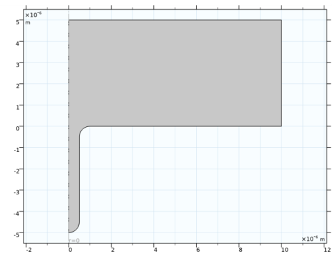
Click in the Graphics window and then press Ctrl+A to select both objects.
|
|
3
|
|
4
|
|
5
|
|
1
|
|
2
|
|
3
|
On the object uni1, select Points 4 and 5 only.
|
|
4
|
|
5
|
|
6
|
|
1
|
In the Model Builder window, under Component 1 (comp1) click Tertiary Current Distribution, Nernst-Planck (tcd).
|
|
2
|
In the Settings window for Tertiary Current Distribution, Nernst-Planck, locate the Electrolyte Charge Conservation section.
|
|
3
|
|
1
|
In the Model Builder window, under Component 1 (comp1) right-click Definitions and choose Variables.
|
|
2
|
|
3
|
|
4
|
Browse to the model’s Application Libraries folder and double-click the file pitting_corrosion_variables.txt.
|
|
1
|
|
2
|
|
3
|
|
4
|
|
5
|
|
6
|
|
7
|
|
8
|
|
9
|
|
10
|
|
11
|
|
12
|
|
1
|
|
2
|
|
3
|
|
4
|
|
5
|
|
1
|
|
3
|
|
4
|
|
5
|
|
6
|
|
7
|
|
8
|
|
9
|
|
1
|
|
1
|
|
3
|
In the Settings window for Electrode Surface, click to expand the Dissolving-Depositing Species section.
|
|
4
|
Click
|
|
6
|
|
7
|
|
1
|
|
2
|
|
3
|
|
4
|
|
5
|
In the Stoichiometric coefficients for dissolving-depositing species: table, enter the following settings:
|
|
6
|
|
7
|
|
8
|
|
1
|
In the Model Builder window, under Component 1 (comp1)>Tertiary Current Distribution, Nernst-Planck (tcd) click Initial Values 1.
|
|
2
|
|
3
|
|
4
|
|
5
|
|
1
|
In the Model Builder window, under Component 1 (comp1)>Multiphysics click Nondeforming Boundary 1 (ndbdg1).
|
|
2
|
|
3
|
|
1
|
In the Model Builder window, under Component 1 (comp1) click Tertiary Current Distribution, Nernst-Planck (tcd).
|
|
2
|
In the Settings window for Tertiary Current Distribution, Nernst-Planck, click to expand the Discretization section.
|
|
3
|
|
4
|
|
5
|
|
1
|
|
2
|
|
3
|
|
1
|
|
2
|
|
3
|
|
5
|
|
1
|
|
2
|
|
3
|
|
5
|
|
6
|
|
1
|
|
2
|
|
3
|
|
4
|
|
5
|
|
1
|
|
1
|
|
2
|
|
3
|
|
4
|
|
5
|
Click to expand the Study Extensions section. Use automatic remeshing to stop and remesh the model if the mesh gets too distorted due to the geometry deformation.
|
|
6
|
|
7
|
|
1
|
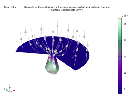
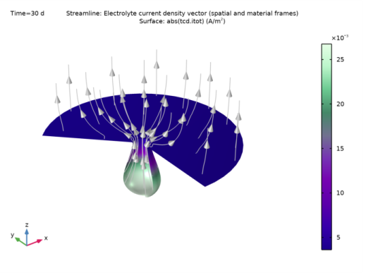
In the Model Builder window, expand the Results>Electrolyte Current Density, 3D (tcd) node, then click Electrolyte Current Density, 3D (tcd).
|
|
2
|
|
3
|
|
1
|
|
2
|
|
3
|
|
4
|
Locate the Coloring and Style section. Find the Point style subsection. From the Arrow length list, choose Normalized.
|
|
1
|
|
2
|
|
1
|
|
2
|
|
3
|
|
4
|
|
5
|
|
6
|
|
7
|
|
1
|
|
2
|
|
3
|
|
4
|
|
1
|
|
2
|
|
3
|
|
4
|
|
1
|
|
2
|
|
1
|
|
2
|
|
3
|
|
1
|
|
2
|
|
3
|
|
1
|
|
2
|
|
3
|
|
1
|
|
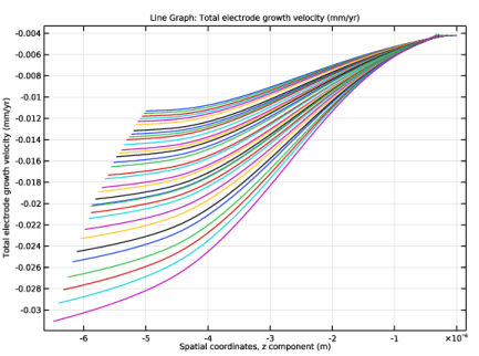
3
|
In the Settings window for Line Graph, click Replace Expression in the upper-right corner of the y-Axis Data section. From the menu, choose Component 1 (comp1)>Tertiary Current Distribution, Nernst-Planck>Dissolving-depositing species>tcd.vbtot - Total electrode growth velocity - m/s.
|
|
4
|
|
5
|
|
6
|
|
7
|
|
1
|
|
2
|
|
3
|
|
4
|
|
5
|