|
|
|

|
1
|
|
2
|
In the Select Physics tree, select Electrochemistry>Tertiary Current Distribution, Nernst-Planck>Tertiary, Supporting Electrolyte (tcd).
|
|
3
|
Click Add.
|
|
4
|
|
5
|
In the Concentrations table, enter the following settings:
|
|
6
|
|
7
|
Click Add.
|
|
8
|
Click
|
|
9
|
|
10
|
Click
|
|
1
|
|
2
|
|
3
|
|
4
|
Browse to the model’s Application Libraries folder and double-click the file oxide_jacking_parameters.txt.
|
|
1
|
|
2
|
|
3
|
|
4
|
Click to expand the Layers section. In the table, enter the following settings:
|
|
5
|
|
6
|
|
1
|
|
2
|
|
3
|
|
4
|
|
5
|
|
6
|
|
1
|
|
2
|
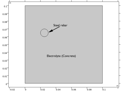
On the object fin, select Domains 1, 3, and 4 only.
|
|
3
|
|
1
|
|
2
|
|
3
|
|
4
|
|
5
|
|
6
|
Click OK.
|
|
1
|
|
2
|
|
3
|
|
4
|
Browse to the model’s Application Libraries folder and double-click the file oxide_jacking_variables.txt.
|
|
1
|
|
2
|
|
3
|
|
4
|
|
5
|
Browse to the model’s Application Libraries folder and double-click the file oxide_jacking_sigma.txt.
|
|
6
|
|
1
|
|
2
|
|
3
|
|
4
|
|
5
|
Browse to the model’s Application Libraries folder and double-click the file oxide_jacking_D_O2.txt.
|
|
6
|
|
1
|
|
2
|
|
3
|
|
4
|
|
1
|
|
2
|
|
3
|
|
1
|
|
2
|
In the tree, select Built-in>Concrete.
|
|
3
|
|
1
|
|
2
|
|
3
|
|
4
|
Click OK.
|
|
6
|
|
1
|
|
2
|
|
3
|
|
1
|
In the Model Builder window, under Component 1 (comp1)>Tertiary Current Distribution, Nernst-Planck (tcd) click Electrolyte 1.
|
|
2
|
|
3
|
|
4
|
Locate the Electrolyte Current Conduction section. From the σl list, choose User defined. In the associated text field, type sigma(PS).
|
|
1
|
|
3
|
|
4
|
|
5
|
|
1
|
|
3
|
In the Settings window for Electrode Surface, click to expand the Dissolving-Depositing Species section.
|
|
4
|
Click
|
|
6
|
Click
|
|
1
|
In the Model Builder window, under Component 1 (comp1)>Tertiary Current Distribution, Nernst-Planck (tcd)>Electrode Surface 1 click Electrode Reaction 1.
|
|
2
|
|
3
|
|
4
|
|
5
|
Locate the Equilibrium Potential section. From the Eeq list, choose User defined. In the associated text field, type Eeq_O2.
|
|
6
|
Locate the Electrode Kinetics section. From the Kinetics expression type list, choose Cathodic Tafel equation.
|
|
7
|
|
8
|
|
1
|
|
2
|
|
3
|
|
4
|
|
5
|
In the Stoichiometric coefficients for dissolving-depositing species: table, enter the following settings:
|
|
6
|
Locate the Equilibrium Potential section. From the Eeq list, choose User defined. In the associated text field, type Eeq_Fe.
|
|
7
|
Locate the Electrode Kinetics section. From the Kinetics expression type list, choose Anodic Tafel equation.
|
|
8
|
|
9
|
|
1
|
|
2
|
|
3
|
Locate the Equilibrium Potential section. From the Eeq list, choose User defined. In the associated text field, type Eeq_H2.
|
|
4
|
Locate the Electrode Kinetics section. From the Kinetics expression type list, choose Cathodic Tafel equation.
|
|
5
|
|
6
|
|
1
|
In the Model Builder window, under Component 1 (comp1)>Tertiary Current Distribution, Nernst-Planck (tcd) click Initial Values 1.
|
|
2
|
|
3
|
|
1
|
|
2
|
|
3
|
|
1
|
|
1
|
|
2
|
|
3
|
Find the Damage evolution subsection. From the σts list, choose User defined. In the associated text field, type sigmap.
|
|
4
|
|
5
|
|
6
|
|
7
|
|
1
|
|
1
|
|
2
|
|
3
|
|
5
|
|
1
|
|
2
|
|
1
|
|
2
|
|
3
|
|
4
|
|
1
|
|
2
|
|
3
|
|
4
|
|
5
|
|
6
|
|
7
|
In the Model Builder window, expand the Study 1>Solver Configurations>Solution 1 (sol1)>Time-Dependent Solver 1 node, then click Fully Coupled 1.
|
|
8
|
|
9
|
|
10
|
|
11
|
|
12
|
|
1
|
|
2
|
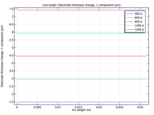
In the Settings window for 1D Plot Group, type Corrosion Product Layer Thickness in the Label text field.
|
|
3
|
|
4
|
|
1
|
|
3
|
In the Settings window for Line Graph, click Replace Expression in the upper-right corner of the y-Axis Data section. From the menu, choose Component 1 (comp1)>Tertiary Current Distribution, Nernst-Planck>Dissolving-depositing species>Electrode thickness change - m>tcd.sb_oxide - Electrode thickness change, 1 component.
|
|
4
|
|
5
|
|
6
|
|
1
|
|
2
|
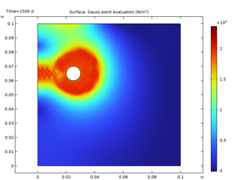
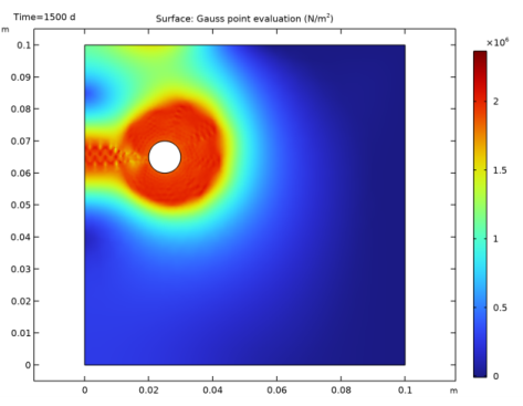
In the Settings window for 2D Plot Group, type First Principal Stress Analysis in the Label text field.
|
|
1
|
|
2
|
|
3
|
|
4
|
|
1
|
|
2
|
|
1
|
|
2
|
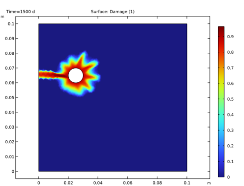
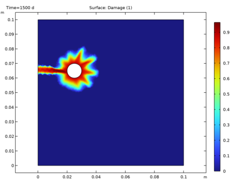
In the Settings window for Surface, click Replace Expression in the upper-right corner of the Expression section. From the menu, choose Component 1 (comp1)>Solid Mechanics>Damage>solid.dmg - Damage.
|
|
1
|
|
2
|
|
1
|
|
2
|
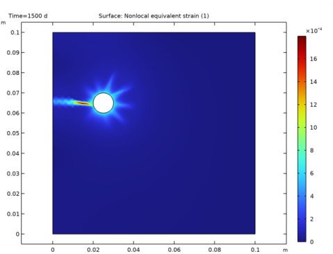
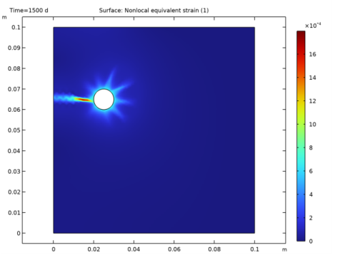
In the Settings window for Surface, click Replace Expression in the upper-right corner of the Expression section. From the menu, choose Component 1 (comp1)>Solid Mechanics>Damage>solid.eeqnl - Nonlocal equivalent strain.
|
|
3
|