|
|
|
|
1
|
|
2
|
|
3
|
Click Add.
|
|
4
|
Click
|
|
5
|
|
6
|
Click
|
|
1
|
|
2
|
|
3
|
|
4
|
Browse to the model’s Application Libraries folder and double-click the file monopile_parameters.txt.
|
|
1
|
|
2
|
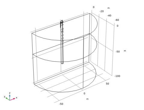
Browse to the model’s Application Libraries folder and double-click the file monopile_geom_sequence.mph.
|
|
3
|
|
4
|
|
5
|
|
1
|
|
2
|
|
3
|
In the tree, select Corrosion>Electrolytes>Seawater.
|
|
4
|
|
5
|
|
1
|
|
2
|
|
1
|
|
2
|
|
4
|
|
1
|
|
2
|
|
3
|
|
4
|
|
1
|
|
2
|
|
3
|
|
4
|
|
5
|
|
6
|
|
7
|
|
1
|
|
2
|
|
3
|
|
4
|
|
5
|
|
1
|
|
2
|
|
3
|
|
4
|
|
1
|
|
2
|
|
3
|
|
4
|
|
5
|
|
6
|
|
7
|
Click OK.
|
|
1
|
|
2
|
|
3
|
|
4
|
|
1
|
|
2
|
In the Settings window for Protected Metal Surface, type Protected Metal Surface - Coated Steel in the Label text field.
|
|
3
|
|
4
|
|
1
|
|
2
|
In the Settings window for Electrode Surface, type Electrode Surface - Uncoated Steel in the Label text field.
|
|
3
|
|
1
|
|
2
|
In the Settings window for Electrode Reaction, type Electrode Reaction 1 - Steel Oxidation in the Label text field.
|
|
3
|
|
4
|
Locate the Electrode Kinetics section. From the Kinetics expression type list, choose Anodic Tafel equation.
|
|
5
|
|
6
|
|
1
|
|
2
|
In the Settings window for Electrode Reaction, type Electrode Reaction 2 - Oxygen Reduction (Sea) in the Label text field.
|
|
3
|
|
4
|
|
5
|
Locate the Electrode Kinetics section. From the iloc,expr list, choose User defined. In the associated text field, type ilim_O2.
|
|
1
|
|
2
|
In the Settings window for Electrode Reaction, type Electrode Reaction 3 - Oxygen Reduction (Mud) in the Label text field.
|
|
3
|
|
4
|
|
1
|
|
2
|
|
3
|
|
4
|
|
5
|
|
6
|
|
1
|
|
2
|
|
3
|
|
1
|
|
1
|
|
2
|
|
3
|
|
1
|
In the Model Builder window, under Component 1 (comp1) right-click Mesh 1 and choose Edit Physics-Induced Sequence.
|
|
2
|
|
3
|
Click the Custom button.
|
|
4
|
|
5
|
|
1
|
|
2
|
|
3
|
|
4
|
|
5
|
|
6
|
Click the Custom button.
|
|
7
|
|
9
|
|
1
|
|
2
|
|
3
|
|
4
|
|
5
|
|
6
|
|
7
|
|
8
|
|
1
|
|
2
|
|
3
|
|
4
|
|
1
|
|
2
|
|
3
|
|
4
|
|
1
|
|
2
|
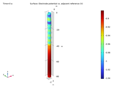
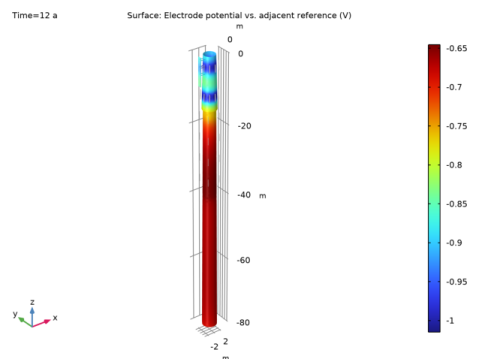
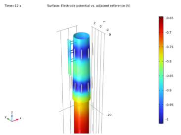
In the Settings window for Surface, click Replace Expression in the upper-right corner of the Expression section. From the menu, choose Component 1 (comp1)>Cathodic Protection>cp.Evsref - Electrode potential vs. adjacent reference - V.
|
|
3
|
|
1
|
|
2
|
|
3
|
|
4
|
|
5
|
|
6
|
|
7
|
|
8
|
|
9
|
|
1
|
|
2
|
|
3
|
|
4
|
|
5
|
|
6
|
|
7
|
|
1
|
|
2
|
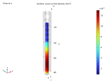
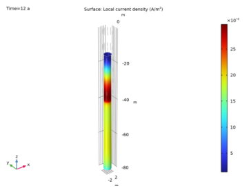
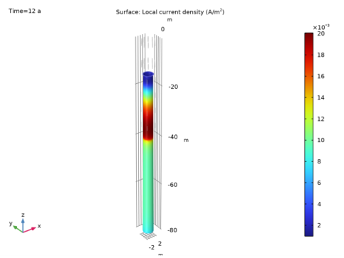
In the Settings window for 3D Plot Group, type Iron Dissolution Current Density in the Label text field.
|
|
1
|
In the Model Builder window, expand the Iron Dissolution Current Density node, then click Surface 1.
|
|
2
|
In the Settings window for Surface, click Replace Expression in the upper-right corner of the Expression section. From the menu, choose Component 1 (comp1)>Cathodic Protection>Electrode kinetics>cp.iloc_er1 - Local current density - A/m².
|
|
3
|
|
4
|
|
1
|
|
2
|
|
3
|
|
4
|
|
5
|
|
6
|
|
1
|
In the Model Builder window, under Component 1 (comp1)>Cathodic Protection (cp) click Electrode Surface - Uncoated Steel.
|
|
2
|
In the Settings window for Electrode Surface, locate the Electrode Phase Potential Condition section.
|
|
3
|
|
4
|
|
1
|
|
2
|
|
1
|
|
2
|
Click
|
|
1
|
|
2
|
|
3
|
|
4
|
|
5
|
|
6
|
|
7
|
|
8
|
|
1
|
|
2
|
|
3
|
|
4
|
|
5
|
|
6
|
|
7
|
|
1
|
|
2
|
|
3
|
|
4
|
|
5
|
Click to expand the Local Coordinate System section. Click to collapse the Local Coordinate System section.
|
|
1
|
|
2
|
|
3
|
|
4
|
|
5
|
|
6
|
|
7
|
|
8
|
|
1
|
|
2
|
|
3
|
|
4
|
|
5
|
|
6
|
|
7
|
|
8
|
|
9
|
|
10
|
|
1
|
|
2
|
|
3
|
|
1
|
|
2
|
|
3
|
|
4
|
|
5
|
|
6
|
|
1
|
|
2
|
|
1
|
|
2
|
In the tree, select wp2>1.
|
|
3
|
|
4
|
|
5
|
|
6
|
|
7
|
|
8
|
|
9
|
|
10
|
|
11
|
|
12
|
|
13
|
|
1
|
|
2
|
Select the object swe1 only.
|
|
3
|
|
4
|
|
5
|
|
1
|
|
2
|
|
3
|
|
4
|
|
5
|
|
6
|
|
1
|
|
2
|
|
3
|
|
4
|
|
5
|
|
6
|
|
7
|
|
8
|
|
9
|
|
1
|
|
2
|
|
3
|
|
4
|
|
5
|
|
6
|
|
7
|
|
1
|
|
2
|
|
3
|
|
4
|
|
1
|
|
2
|
|
3
|
|
4
|
|
5
|
|
6
|
|
1
|
|
2
|
|
3
|
|
4
|
|
5
|
|
6
|
|
7
|
|
8
|
|
9
|
|
10
|
|
1
|
|
2
|
|
4
|
|
5
|
|
1
|
|
2
|
|
3
|
|
4
|
|
5
|
|
6
|
|
1
|
|
2
|
|
3
|
|
1
|
|
2
|
In the tree, select cone2 (solid), swe1 (solid), copy1 (solid), cyl1 (solid), Array 1>arr1(1,1,1) (solid), Array 1>arr1(1,1,2) (solid), Array 1>arr1(1,1,3) (solid), Array 1>arr1(1,1,4) (solid), Array 1>arr1(1,1,5) (solid), Array 1>arr1(1,1,6) (solid), Array 1>arr1(1,1,7) (solid), Array 1>arr1(1,1,8) (solid), Array 1>arr1(1,1,9) (solid), Array 1>arr1(1,1,10) (solid), Array 1>arr1(1,1,11) (solid), Array 1>arr1(1,1,12) (solid), Array 1>arr1(1,1,13) (solid), Array 1>arr1(1,1,14) (solid), Array 1>arr1(1,1,15) (solid), Array 1>arr1(1,1,16) (solid), Array 1>arr1(1,1,17) (solid), Array 1>arr1(1,1,18) (solid), Array 1>arr1(1,1,19) (solid), Array 1>arr1(1,1,20) (solid), Array 1>arr1(1,1,21) (solid), Array 1>arr1(1,1,22) (solid), Array 1>arr1(1,1,23) (solid), Array 1>arr1(1,1,24) (solid), Array 1>arr1(1,1,25) (solid), Array 1>arr1(1,1,26) (solid), Array 1>arr1(1,1,27) (solid), Array 1>arr1(1,1,28) (solid), Array 1>arr1(1,1,29) (solid), Array 1>arr1(1,1,30) (solid), Array 1>arr1(1,1,31) (solid), Array 1>arr1(1,1,32) (solid), Array 1>arr1(1,1,33) (solid), Array 1>arr1(1,1,34) (solid), Array 1>arr1(1,1,35) (solid), Array 1>arr1(1,1,36) (solid), Array 1>arr1(1,1,37) (solid), Array 1>arr1(1,1,38) (solid), Array 1>arr1(1,1,39) (solid), Array 1>arr1(1,1,40) (solid), Array 1>arr1(1,1,41) (solid), Array 1>arr1(1,1,42) (solid), Array 1>arr1(1,1,43) (solid), Array 1>arr1(1,1,44) (solid), Array 1>arr1(1,1,45) (solid), Array 1>arr1(1,1,46) (solid), Array 1>arr1(1,1,47) (solid), Array 1>arr1(1,1,48) (solid), Array 1>arr1(1,1,49) (solid), Array 1>arr1(1,1,50) (solid), and mov1 (solid).
|
|
3
|
|
1
|
|
2
|
|
1
|
|
2
|
|
3
|
|
4
|
|
5
|
|
6
|
Click to expand the Layers section. In the table, enter the following settings:
|
|
7
|
|
8
|
|
9
|
|
1
|
|
2
|
|
3
|
|
4
|
|
5
|
|
6
|
|
7
|
|
8
|
|
9
|
|
1
|
|
2
|
|
3
|
|
4
|
|
5
|
|
6
|
|
7
|
|
8
|
|
1
|
|
2
|
|
1
|
|
2
|
|
3
|
|
4
|
On the object dif1, select Domains 4–7 only.
|
|
1
|
|
2
|
|
1
|
|
2
|
|
4
|
Locate the Selections of Resulting Entities section. Find the Cumulative selection subsection. Click New.
|
|
5
|
|
6
|
Click OK.
|
|
1
|
|
2
|
|
3
|
|
4
|
Locate the Rotation section. In the Angle text field, type -range(180/NanodeTp,360/NanodeTp,180-180/NanodeTp).
|
|
5
|
Locate the Selections of Resulting Entities section. Find the Cumulative selection subsection. From the Contribute to list, choose AnodeTp.
|
|
6
|
|
1
|
|
2
|
|
3
|
|
4
|
In the Paste Selection dialog box, type rot1(1) rot1(2) rot1(3) rot1(4) rot1(5) in the Selection text field.
|
|
5
|
Click OK.
|
|
6
|
|
7
|
|
8
|
|
9
|
Locate the Selections of Resulting Entities section. Find the Cumulative selection subsection. From the Contribute to list, choose AnodeTp.
|
|
10
|
|
1
|
|
2
|
|
3
|
|
4
|
|
5
|
|
6
|
|
7
|
Locate the Selections of Resulting Entities section. Find the Cumulative selection subsection. Click New.
|
|
8
|
|
9
|
Click OK.
|
|
1
|
|
2
|
|
3
|
|
4
|
|
5
|
|
6
|
|
1
|
|
2
|
|
3
|
|
4
|
In the Paste Selection dialog box, type arr2(1,1,1) arr2(1,1,2) arr2(1,1,3) arr2(1,1,4) in the Selection text field.
|
|
5
|
Click OK.
|
|
6
|
|
7
|
|
8
|
|
9
|
Locate the Selections of Resulting Entities section. Find the Cumulative selection subsection. From the Contribute to list, choose AnoodeMp.
|
|
10
|
|
1
|
|
2
|
|
3
|
|
4
|
|
5
|
|
6
|
Click OK.
|
|
1
|
|
2
|
|
3
|
|
4
|
In the Paste Selection dialog box, type del1 rot1(1) rot1(2) rot1(3) rot1(4) rot1(5) copy2(1) copy2(2) copy2(3) copy2(4) copy2(5) del1 rot1(1) rot1(2) rot1(3) rot1(4) rot1(5) rot2(1) rot2(2) rot2(3) rot2(4) rot2(5) rot2(6) rot2(7) rot2(8) in the Selection text field.
|
|
5
|
Click OK.
|
|
6
|
Click in the Graphics window and then press Ctrl+A to select all objects.
|
|
7
|
|
8
|
|
9
|