Stefan Tube

This example illustrates the use of the Maxwell-Stefan diffusion model available with the Transport of Concentrated Species interface. It models multicomponent gas-phase diffusion in a Stefan tube in 1D. In this case, it is a liquid mixture of acetone and methanol that evaporates into air.

The concentration profiles are modeled at steady-state and validated against experimental data by Taylor and Krishna (Ref. 6).

Model Definition

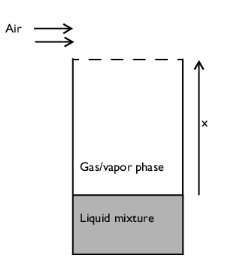
The Stefan tube, shown in Figure 1, is a simple device used for measuring diffusion coefficients in binary vapors.

Figure 1: Schematic diagram of a Stefan tube.

At the bottom of the tube is a pool of mixture. The vapor that evaporates from this pool diffuses to the top of the tube, where a stream of air, flowing across the top of the tube, keeps the mole fraction of diffusing vapor there to be zero. The mole fraction of vapor above the liquid interface is at equilibrium. Because there is no horizontal flux inside the tube, you can analyze the problem using a 1D model geometry representing the distance between the liquid mixture surface and the top of the tube. The system composition of acetone, methanol, and air has been extensively investigated; both diffusion coefficients and composition have been measured at various positions within Stefan tubes. This makes it an ideal system for this model.

As a comparison, one experiment measured the mole fraction at the liquid interface to be xAc = 0.319 and xMe = 0.528 where the pressure, p, was 99.4 kPa and the temperature, T, was 328.5 K. The length of the diffusion path was 0.238 m. The respective Maxwell-Stefan diffusion coefficients, Dij, of the three binary pairs were calculated and are used in the model according to Table 1.

Table 1: labels and Maxwell-Stefan diffusion coefficients.
component	label	Dij	value
Acetone	1	D12	8.48·10-6 m2/s
Methanol	2	D13	13.72·10-6 m2/s
Air	3	D23	19.91·10-6 m2/s

To model this problem, use the Transport of Concentrated Species interface with the Maxwell-Stefan diffusion model. It solves for the fluxes in terms of mass fractions for two of the three components. The mass fraction, ω, of the third is given by the two other ones. The three equations are:

where Dij are the is the multicomponent Fick diffusivities (SI unit: m2/s), p is the pressure (SI unit: Pa), T is the temperature (SI unit: K), u is the velocity (SI unit: m/s), x and ω are mole and mass fractions, respectively, and the mixture density, ρmix (SI unit: kg/m3), is a function of the average mixture mole fraction, Mmix (SI unit: kg/mol), according to Equation 2:

(1)

(2)

In this case, there is no imposed fluid velocity. However, a mixture velocity will result due to the mass transfer from liquid mixture. At the top of the tube the mass fractions are fixed, with the fraction of air being unity. At the bottom (at the liquid interface), the fractions are also fixed according to the previously mentioned experimental conditions. The fact that there is no air flux at the interface results in the following relation for the convective velocity, at steady state:

where ndiff,3 is the diffusive mass flux of air (SI unit: kg/(m2·s)).

Results

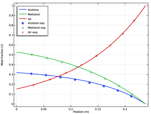
Both the modeled and experimental steady-state mole fractions as a function of position are shown in Figure 2.

Figure 2: Modeled and experimental (Ref. 6) steady-state mole fractions of: acetone, methanol, and air, in the Stefan tube.

We can see that the model reproduces the results from Ref. 6 well, which means the Maxwell-Stefan equations can describe the mass transport process in the system accurately.

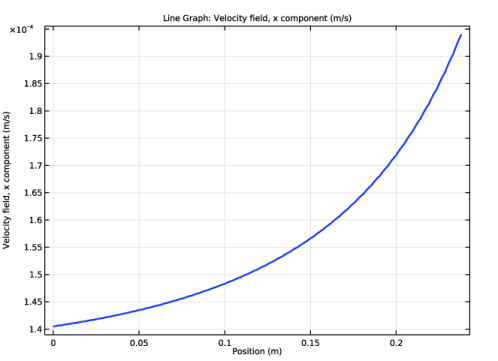
The Maxwell-Stefan diffusion formulation includes the conservation of mass. In the absence of chemical reactions (source terms) and convective contributions, the Maxwell-Stefan formulation results in zero net mass flux. In this example, the convective term is included, which you can see in the velocity profile in Figure 3.

References

1. C.F. Curtiss and R.B. Bird, “Multicomponent diffusion,” Ind. Eng. Chem. Res., vol. 38, p. 2515, 1999.
2. R.B. Bird, W. Stewart, and E. Lightfoot, Transport Phenomena, John Wiley & Sons, New York, 1960.
3. G.A.J. Jaumann, Wien. Akad. Sitzungsberichte (Math.-Naturw. Klasse), vol. 120, p. 385, 1911.
4. J.O. Hirschfelder, C.F. Curtiss, and R.B. Bird, Molecular Theory of Gases and Liquids, Wiley, USA, 1954.
5. E.N. Fuller, P.D. Schettler, and J.C. Giddings, Ind. Eng. Chem., vol. 58, p. 19, 1966.
6. R. Taylor and R. Krishna, Multicomponent Mass Transfer, John Wiley & Sons, NY, p. 21, 1993.
Application Library path: Chemical_Reaction_Engineering_Module/Mixing_and_Separation/stefan_tube
Modeling Instructions
From the File menu, choose New.
New
In the New window, click  Model Wizard.
Model Wizard
1
In the Model Wizard window, click  1D.
2
In the Select Physics tree, select Chemical Species Transport>Transport of Concentrated Species (tcs).
3
Click Add.
4
Click  Add Mass Fraction.
5
In the Mass fractions table, enter the following settings:
6
Click  Study.
7
In the Select Study tree, select General Studies>Stationary.
8
Geometry 1
Interval 1 (i1)
In the Model Builder window, under Component 1 (comp1) right-click Geometry 1 and choose Interval.
In the Settings window for Interval, locate the Interval section.
Click  Build All Objects.
Global Definitions
Next, add a set of model parameters by importing their definitions from a data text file provided with the Application Library.
Parameters 1
In the Model Builder window, under Global Definitions click Parameters 1.
In the Settings window for Parameters, locate the Parameters section.
Click  Load from File.
Transport of Concentrated Species (tcs)
In the Model Builder window, under Component 1 (comp1) click Transport of Concentrated Species (tcs).
In the Settings window for Transport of Concentrated Species, locate the Transport Mechanisms section.
From the Diffusion model list, choose Maxwell-Stefan.
Locate the Species section. From the From mass constraint list, choose w3.
Click to expand the Discretization section. From the Mass fraction list, choose Quadratic.
Transport Properties 1
In the Model Builder window, under Component 1 (comp1)>Transport of Concentrated Species (tcs) click Transport Properties 1.
In the Settings window for Transport Properties, locate the Model Input section.
From the T list, choose User defined. In the associated text field, type T0.
From the pA list, choose User defined. In the associated text field, type p0.
Locate the Convection section. Specify the u vector as
Locate the Density section. In the Mw1 text field, type M_ace.
In the Mw2 text field, type M_met.
In the Mw3 text field, type M_air.
9
Locate the Diffusion section. In the table, enter the following settings:
Initial Values 1
In the Model Builder window, click Initial Values 1.
In the Settings window for Initial Values, locate the Initial Values section.
In the ω0,w1 text field, type w_ace0.
In the ω0,w2 text field, type w_met0.
Mass Fraction 1
In the Physics toolbar, click  Boundaries and choose Mass Fraction.
In the Settings window for Mass Fraction, locate the Mass Fraction section.
Select the Species w1 check box.
Select the Species w2 check box.
Mass Fraction 2
Mesh 1
In the Model Builder window, under Component 1 (comp1) click Mesh 1.
In the Settings window for Mesh, locate the Physics-Controlled Mesh section.
From the Element size list, choose Extra fine.
Click  Build All.
Study 1
In the Home toolbar, click  Compute.
Results
Experimental Mole Fractions
In the Results toolbar, click  Table.
Import the experimental data for comparison.
In the Settings window for Table, type Experimental Mole Fractions in the Label text field.
Locate the Data section. Click Import.
In order to reproduce the plot in Figure 2, do the following:
Mole Fractions, All Species
In the Results toolbar, click  1D Plot Group.
In the Settings window for 1D Plot Group, type Mole Fractions, All Species in the Label text field.
Line Graph 1
Right-click Mole Fractions, All Species and choose Line Graph.
In the Settings window for Line Graph, locate the Selection section.
From the Selection list, choose All domains.
Click to expand the Title section. Click Replace Expression in the upper-right corner of the y-Axis Data section. From the menu, choose Component 1 (comp1)>Transport of Concentrated Species>Species w1>tcs.x_w1 - Mole fraction.
Locate the Title section. From the Title type list, choose None.
Locate the x-Axis Data section. From the Parameter list, choose Expression.
In the Expression text field, type x.
Click to expand the Coloring and Style section. In the Width text field, type 2.
Click to expand the Legends section. Select the Show legends check box.
10
From the Legends list, choose Manual.
11
Line Graph 2
Right-click Line Graph 1 and choose Duplicate.
In the Settings window for Line Graph, click Replace Expression in the upper-right corner of the y-Axis Data section. From the menu, choose Component 1 (comp1)>Transport of Concentrated Species>Species w2>tcs.x_w2 - Mole fraction.
Locate the Legends section. In the table, enter the following settings:
Line Graph 3
Right-click Line Graph 2 and choose Duplicate.
In the Settings window for Line Graph, click Replace Expression in the upper-right corner of the y-Axis Data section. From the menu, choose Component 1 (comp1)>Transport of Concentrated Species>Species w3>tcs.x_w3 - Mole fraction.
Table Graph 1
In the Model Builder window, right-click Mole Fractions, All Species and choose Table Graph.
In the Settings window for Table Graph, locate the Data section.
From the x-axis data list, choose Column 1.
Locate the Coloring and Style section. Find the Line markers subsection. From the Marker list, choose Cycle.
Find the Line style subsection. From the Line list, choose None.
From the Color list, choose Cycle (reset).
In the Model Builder window, click Mole Fractions, All Species.
In the Settings window for 1D Plot Group, locate the Plot Settings section.
Select the x-axis label check box.
Locate the Legend section. From the Position list, choose Upper left.
To reproduce Figure 3, proceed as follows:
Velocity Field
In the Settings window for 1D Plot Group, type Velocity Field in the Label text field.
Locate the Plot Settings section. Select the x-axis label check box.
Right-click Velocity Field and choose Line Graph.
In the Settings window for Line Graph, click Replace Expression in the upper-right corner of the y-Axis Data section. From the menu, choose Component 1 (comp1)>Transport of Concentrated Species>Velocity field - m/s>tcs.u - Velocity field, x component.
Locate the Coloring and Style section. In the Width text field, type 2.
In the Velocity Field toolbar, click  Plot.