You are viewing the documentation for an older COMSOL version. The latest version is available here.
PDF

Porous Reactor with Injection Needle
Introduction
This example treats the flow field and species distribution in an experimental reactor for studies of heterogeneous catalysis. The application gives an example of the coupling of free and porous media flow in fixed bed reactors. The model was inspired by numerical experiments performed by Professor Finlayson’s graduate students in chemical engineering at the University of Washington in Seattle.
Model Definition
The reactor consists of a tubular structure with an injection tube whose main axis is perpendicular to the reactor axis. The incoming species in the main and injection tubes react in a fixed porous catalyst bed. The model couples the free fluid and porous media flow through the Reacting Flow in Porous Media interface. This physics interface supports both free-flow domains and porous-media domains.
Because of symmetry, only one half of the reactor is modeled; see Figure 1.
Figure 1: The species A and B enter the reactor from the main and injection tubes, respectively, and react in a fixed porous catalyst bed to produce C.
In the porous bed, a reaction takes place that consumes species A and B and produces C: .
Governing Equations
The stationary Navier-Stokes equations describe the fluid flow in the free-flow regions. In the porous bed, the Brinkman equations for porous media apply.
A Fickian approach for the diffusion term in the mass transport can be utilized by assuming that the modeled species are present in low concentrations compared to the solvent gas. The mass transport for the three species A, B, and C can therefore be modeled with the convection-diffusion equation
In this equation, ci denotes the concentration (SI unit: mol/m3), Di the diffusivity (SI unit: m2 /s), and Ri the reaction rate for species i (SI unit: mol/(m3·s)). Because the reaction takes place in the porous bed only, the reaction term is zero in the free-flow regions. The reaction is a second order irreversible reaction and the rates are given by
where kf is the reaction rate constant, which in turn is temperature dependent according to the Arrhenius law:
Where Af is the frequency factor (SI unit: m3/(mol·s)), Ea is the activation energy (SI unit: J/mol), R the universal gas constant (SI unit: J/(mol·K)), and T the local temperature (SI unit: K). The following data are used for the reaction:
Table 1: Data.
Af
1·106 m3/(mol·s)
Ea
30·103 J/mol
R_const (built in constant)
Boundary Conditions
A constant velocity profile is assumed at the inlet boundaries
For the outlet, a pressure condition is applied.
In the mass transport, the concentrations at the inlet are fixed
At the outlet, the convection is assumed to dominate the mass transport
This implies that the gradient of ci in the direction perpendicular to the outlet boundary is negligible. This is a common assumption for tubular reactors with a high degree of transport by convection in the direction of the main reactor axis. The condition eliminates the need for specifying a concentration or a fixed value for the flux at the outlet boundary. At all other boundaries, insulating conditions apply
Results and Discussion
Figure 2 shows the velocity magnitude. The flow is almost homogeneous in the porous part of the reactor.
Figure 2: Magnitude of the velocity field in the free and porous reactor domains.
Figure 3 shows the pressure drop, which occurs mainly across the porous bed.
Figure 3: The pressure drop across the reactor.
Figure 4 and Figure 5 show the concentrations of species A and B, respectively.
Figure 4: Isoconcentration surfaces for species A.
Figure 5: Isoconcentration surfaces for species B.
Figure 4 shows that the concentration of the injected species A decays very rapidly with the distance from the injection point. This implies that the porous bed is not optimally used. Figure 5 shows the isoconcentration surfaces of species B, which is introduced in the main channel of the reactor. The reaction is not uniformly distributed in the catalytic bed and has its maximum close to the radial position of the injection pipe. The low concentration of B at the injection point is due to dilution by the solvent that carries species A.
In summary, the model shows that the injection point is far too close to the porous bed. The reactants are not well mixed and only a fraction of the bed is utilized. A proper design should include a small static mixer after the injection point or a positioning of the injection point further upstream in order to obtain mixing through diffusion.
Application Library path: Chemical_Reaction_Engineering_Module/Reactors_with_Porous_Catalysts/porous_reactor
Modeling Instructions
From the File menu, choose New.
New
In the New window, click  Model Wizard.
Model Wizard
1
In the Model Wizard window, click  3D.
2
In the Select Physics tree, select Chemical Species Transport>Reacting Flow in Porous Media>Transport of Diluted Species.
3
Click Add.
4
In the Added physics interfaces tree, select Transport of Diluted Species in Porous Media (tds).
5
In the Number of species text field, type 3.
6
In the Concentrations table, enter the following settings:
7
Click  Study.
8
In the Select Study tree, select General Studies>Stationary.
9
Global Definitions
Parameters 1
1
In the Model Builder window, under Global Definitions click Parameters 1.
2
In the Settings window for Parameters, locate the Parameters section.
3
Click  Load from File.
4
Create the geometry. To simplify this step, insert a prepared geometry sequence. In the Geometry toolbar, click Insert Sequence. Browse to the model’s Application Libraries folder and double-click the file porous_reactor.mph. Then click Build All In the Geometry toolbar.
Definitions (comp1)
Catalyst bed
1
In the Definitions toolbar, click  Explicit.
2
Right-click Explicit 1 and choose Rename.
3
In the Rename Explicit dialog box, type Catalyst bed in the New label text field.
4
5
Symmetry plane
1
In the Definitions toolbar, click  Explicit.
2
In the Model Builder window, right-click Explicit 2 and choose Rename.
3
In the Rename Explicit dialog box, type Symmetry plane in the New label text field.
4
5
In the Settings window for Explicit, locate the Input Entities section.
6
From the Geometric entity level list, choose Boundary.
7
Inlet species B
1
In the Definitions toolbar, click  Explicit.
2
Right-click Explicit 3 and choose Rename.
3
In the Rename Explicit dialog box, type Inlet species B in the New label text field.
4
5
In the Settings window for Explicit, locate the Input Entities section.
6
From the Geometric entity level list, choose Boundary.
7
Inlet species A
1
In the Definitions toolbar, click  Explicit.
2
In the Model Builder window, right-click Explicit 4 and choose Rename.
3
In the Rename Explicit dialog box, type Inlet species A in the New label text field.
4
5
In the Settings window for Explicit, locate the Input Entities section.
6
From the Geometric entity level list, choose Boundary.
7
Outlet
1
In the Definitions toolbar, click  Explicit.
2
Right-click Explicit 5 and choose Rename.
3
In the Rename Explicit dialog box, type Outlet in the New label text field.
4
5
In the Settings window for Explicit, locate the Input Entities section.
6
From the Geometric entity level list, choose Boundary.
7
Ball 1
1
In the Model Builder window, right-click Selections and choose Ball.
2
In the Settings window for Ball, locate the Geometric Entity Level section.
3
From the Level list, choose Boundary.
4
Locate the Ball Radius section. In the Radius text field, type 15.
5
Click the  Zoom to Selection button in the Graphics toolbar.
Walls and free-porous media interfaces
1
In the Definitions toolbar, click  Difference.
2
In the Settings window for Difference, type Walls and free-porous media interfaces in the Label text field.
3
Locate the Geometric Entity Level section. From the Level list, choose Boundary.
4
Locate the Input Entities section. Under Selections to add, click  Add.
5
In the Add dialog box, select Ball 1 in the Selections to add list.
6
7
In the Settings window for Difference, locate the Input Entities section.
8
Under Selections to subtract, click  Add.
9
In the Add dialog box, in the Selections to subtract list, choose Symmetry plane, Inlet species B, Inlet species A, and Outlet.
10
Variables 1
1
In the Model Builder window, under Component 1 (comp1) right-click Definitions and choose Variables.
2
In the Settings window for Variables, locate the Geometric Entity Selection section.
3
From the Geometric entity level list, choose Domain.
4
From the Selection list, choose Catalyst bed.
5
Locate the Variables section. Click  Load from File.
6
Materials
Note that a Porous Material node has been created automatically when adding an entry from the Reacting Flow in Porous Media branch. Now add Nitrogen from the Material Library to define the fluid properties in the model.
Add Material
From the Home menu, choose Add Material.
Add Material
1
Go to the Add Material window.
2
In the tree, select Liquids and Gases>Gases>Nitrogen.
3
Click Add to Component in the window toolbar.
4
From the Home menu, choose Add Material.
Materials
Nitrogen (mat1)
1
In the Settings window for Material, locate the Geometric Entity Selection section.
2
From the Selection list, choose All domains.
3
In the Model Builder window, expand the Component 1 (comp1)>Materials node.
4
Right-click Component 1 (comp1)>Materials>Nitrogen (mat1) and choose Move Up.
Porous Material 1 (pmat1)
1
In the Model Builder window, click Porous Material 1 (pmat1).
2
3
In the Settings window for Porous Material, locate the Homogenized Properties section.
4
Fluid (pmat1.fluid)
1
In the Model Builder window, expand the Porous Material 1 (pmat1) node, then click Fluid (pmat1.fluid).
2
In the Settings window for Fluid, locate the Fluid Properties section.
3
From the Material list, choose Nitrogen (mat1).
Solid (pmat1.solid)
1
In the Model Builder window, click Solid (pmat1.solid).
2
In the Settings window for Solid, locate the Solid Properties section.
3
In the θs text field, type 0.7.
Global Definitions
Default Model Inputs
1
In the Model Builder window, under Global Definitions click Default Model Inputs.
2
In the Settings window for Default Model Inputs, locate the Browse Model Inputs section.
3
In the tree, select General>Temperature (K) - minput.T.
4
Find the Expression for remaining selection subsection. In the Temperature text field, type T_iso.
Brinkman Equations (br)
1
In the Model Builder window, under Component 1 (comp1) click Brinkman Equations (br).
2
In the Settings window for Brinkman Equations, locate the Physical Model section.
3
Clear the Neglect inertial term (Stokes flow) check box.
Fluid Properties 1
1
In the Physics toolbar, click  Domains and choose Fluid Properties.
2
Inlet 1
1
In the Physics toolbar, click  Boundaries and choose Inlet.
2
3
In the Settings window for Inlet, locate the Boundary Selection section.
4
From the Selection list, choose Inlet species B.
5
Locate the Boundary Condition section. From the list, choose Fully developed flow.
6
Locate the Fully Developed Flow section. In the Uav text field, type 2.5[cm/s].
Inlet 2
1
In the Physics toolbar, click  Boundaries and choose Inlet.
2
In the Settings window for Inlet, locate the Boundary Selection section.
3
From the Selection list, choose Inlet species A.
4
Locate the Boundary Condition section. From the list, choose Fully developed flow.
5
Locate the Fully Developed Flow section. In the Uav text field, type 2.5[cm/s].
Outlet 1
1
In the Physics toolbar, click  Boundaries and choose Outlet.
2
In the Settings window for Outlet, locate the Boundary Selection section.
3
From the Selection list, choose Outlet.
Symmetry 1
1
In the Physics toolbar, click  Boundaries and choose Symmetry.
2
Transport of Diluted Species in Porous Media (tds)
Fluid 1
1
In the Model Builder window, under Component 1 (comp1)>Transport of Diluted Species in Porous Media (tds)>Porous Medium 1 click Fluid 1.
2
In the Settings window for Fluid, locate the Diffusion section.
3
In the DF,cA text field, type 1e-6[m^2/s].
4
In the DF,cB text field, type 1e-6[m^2/s].
5
In the DF,cC text field, type 1e-6[m^2/s].
6
From the Effective diffusivity model list, choose Bruggeman model.
Transport Properties 1
1
In the Physics toolbar, click  Domains and choose Transport Properties.
2
3
In the Settings window for Transport Properties, locate the Diffusion section.
4
In the DcA text field, type 1e-6[m^2/s].
5
In the DcB text field, type 1e-6[m^2/s].
6
In the DcC text field, type 1e-6[m^2/s].
Reactions 1
1
In the Physics toolbar, click  Domains and choose Reactions.
2
In the Settings window for Reactions, locate the Domain Selection section.
3
From the Selection list, choose Catalyst bed.
4
Locate the Reaction Rates section. In the RcA text field, type -k_f*c_A*c_B.
5
In the RcB text field, type -k_f*c_A*c_B.
6
In the RcC text field, type k_f*c_A*c_B.
Symmetry 1
1
In the Physics toolbar, click  Boundaries and choose Symmetry.
2
In the Settings window for Symmetry, locate the Boundary Selection section.
3
From the Selection list, choose Symmetry plane.
Inflow 1
1
In the Physics toolbar, click  Boundaries and choose Inflow.
2
In the Settings window for Inflow, locate the Boundary Selection section.
3
From the Selection list, choose Inlet species B.
4
Locate the Concentration section. In the c0,cB text field, type 1[mol/m^3].
Inflow 2
1
In the Physics toolbar, click  Boundaries and choose Inflow.
2
In the Settings window for Inflow, locate the Boundary Selection section.
3
From the Selection list, choose Inlet species A.
4
Locate the Concentration section. In the c0,cA text field, type 7[mol/m^3].
Outflow 1
1
In the Physics toolbar, click  Boundaries and choose Outflow.
2
In the Settings window for Outflow, locate the Boundary Selection section.
3
From the Selection list, choose Outlet.
Mesh 1
1
In the Model Builder window, under Component 1 (comp1) click Mesh 1.
2
In the Settings window for Mesh, locate the Sequence Type section.
3
From the list, choose User-controlled mesh.
The Size 1 node added by default refines the mesh on boundaries corresponding to walls. Duplicate this node and apply the same settings to the boundaries corresponding to the needle symmetry plane and the needle outlet to refine the mesh on these boundaries as well.
Size 2
1
In the Model Builder window, under Component 1 (comp1)>Mesh 1 right-click Size 1 and choose Duplicate.
2
In the Settings window for Size, locate the Geometric Entity Selection section.
3
Click  Clear Selection.
4
5
6
Click  Build All.
Study 1
In the Home toolbar, click  Compute.
Results
Velocity (br)
The following steps reproduce, in turn, the plots shown in Figure 2, Figure 3, Figure 4, and Figure 5.
Velocity, Surface
1
In the Home toolbar, click  Add Plot Group and choose 3D Plot Group.
2
In the Settings window for 3D Plot Group, type Velocity, Surface in the Label text field.
Surface 1
1
Right-click Velocity, Surface and choose Surface.
2
In the Velocity, Surface toolbar, click  Plot.
3
Click the  Zoom Extents button in the Graphics toolbar.
Pressure (br)
1
Click the  Zoom Extents button in the Graphics toolbar.
2
In the Model Builder window, under Results click Pressure (br).
3
In the Pressure (br) toolbar, click  Plot.
Symmetry surface
1
In the Model Builder window, expand the Results>Datasets node.
2
Right-click Results>Datasets and choose Surface.
3
In the Settings window for Surface, type Symmetry surface in the Label text field.
4
Locate the Selection section. From the Selection list, choose Symmetry plane.
Concentration, c_A, Isosurface
1
In the Results toolbar, click  3D Plot Group.
2
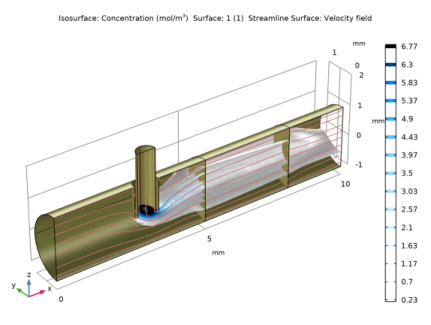
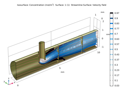
In the Settings window for 3D Plot Group, type Concentration, c_A, Isosurface in the Label text field.
Isosurface 1
1
Right-click Concentration, c_A, Isosurface and choose Isosurface.
2
In the Settings window for Isosurface, click Replace Expression in the upper-right corner of the Expression section. From the menu, choose Component 1 (comp1)>Transport of Diluted Species in Porous Media>Species c_A>c_A - Concentration - mol/m³.
3
Locate the Levels section. In the Total levels text field, type 15.
4
Locate the Coloring and Style section. From the Color table list, choose JupiterAuroraBorealis.
5
From the Color table transformation list, choose Reverse.
Surface 1
1
In the Model Builder window, right-click Concentration, c_A, Isosurface and choose Surface.
2
In the Settings window for Surface, locate the Expression section.
3
In the Expression text field, type 1.
4
Locate the Coloring and Style section. From the Coloring list, choose Uniform.
5
From the Color list, choose Custom.
6
7
Click Define custom colors.
8
9
Click Add to custom colors.
10
Click Show color palette only or OK on the cross-platform desktop.
Selection 1
1
Right-click Surface 1 and choose Selection.
2
In the Settings window for Selection, locate the Selection section.
3
From the Selection list, choose Walls and free-porous media interfaces.
4
In the Concentration, c_A, Isosurface toolbar, click  Plot.
Concentration, c_A, Isosurface
In the Model Builder window, under Results click Concentration, c_A, Isosurface.
Streamline Surface 1
1
In the Concentration, c_A, Isosurface toolbar, click  More Plots and choose Streamline Surface.
2
In the Settings window for Streamline Surface, locate the Data section.
3
From the Dataset list, choose Symmetry surface.
4
Locate the Streamline Positioning section. From the Positioning list, choose Uniform density.
5
In the Separating distance text field, type 0.027.
6
Locate the Coloring and Style section. Find the Line style subsection. From the Type list, choose Tube.
7
In the Tube radius expression text field, type 0.01.
8
Select the Radius scale factor check box.
9
Find the Point style subsection. From the Color list, choose Custom.
10
11
Click Define custom colors.
12
13
Click Add to custom colors.
14
Click Show color palette only or OK on the cross-platform desktop.
15
In the Concentration, c_A, Isosurface toolbar, click  Plot.
16
Click the  Zoom Extents button in the Graphics toolbar.
Concentration, c_B, Isosurface
1
Right-click Concentration, c_A, Isosurface and choose Duplicate.
2
In the Settings window for 3D Plot Group, type Concentration, c_B, Isosurface in the Label text field.
Isosurface 1
1
In the Model Builder window, expand the Concentration, c_B, Isosurface node, then click Isosurface 1.
2
In the Settings window for Isosurface, locate the Expression section.
3
In the Expression text field, type c_B.
4
In the Concentration, c_B, Isosurface toolbar, click  Plot.
Concentration, c_C, Isosurface
1
In the Model Builder window, right-click Concentration, c_B, Isosurface and choose Duplicate.
2
In the Settings window for 3D Plot Group, type Concentration, c_C, Isosurface in the Label text field.
Isosurface 1
1
In the Model Builder window, expand the Concentration, c_C, Isosurface node, then click Isosurface 1.
2
In the Settings window for Isosurface, locate the Expression section.
3
In the Expression text field, type c_C.
4
In the Concentration, c_C, Isosurface toolbar, click  Plot.