
|
|
|


|
k1
|
7.07·1013
|
|
|
k2
|
1.47·1015
|
|
|
KCO
|
||
|
KC3H6
|


|
1
|
In the Model Wizard window, Start by adding the necessary 1D physics interfaces: Transport of Diluted Species and Coefficient Form PDE.
|
|
2
|
click
|
|
3
|
|
4
|
Click Add.
|
|
5
|
|
6
|
In the Concentrations table, enter the following settings:
|
|
7
|
|
8
|
Click Add.
|
|
9
|
|
10
|
In the Dependent variables table, enter the following settings:
|
|
11
|
Click
|
|
12
|
|
13
|
Click
|
|
1
|
|
2
|
|
4
|
|
1
|
|
2
|
|
3
|
|
4
|
Browse to the model’s Application Libraries folder and double-click the file packed_bed_reactor_parameters.txt.
|
|
1
|
|
2
|
|
3
|
|
4
|
Browse to the model’s Application Libraries folder and double-click the file packed_bed_reactor_variables_global.txt.
|
|
1
|
In the Model Builder window, under Component 1 (comp1)>Transport of Diluted Species (tds) click Transport Properties 1.
|
|
2
|
|
3
|
Specify the u vector as
|
|
4
|
|
5
|
|
6
|
|
7
|
|
8
|
|
1
|
|
2
|
|
3
|
|
4
|
|
5
|
|
6
|
|
7
|
|
1
|
|
3
|
|
4
|
|
5
|
|
6
|
|
7
|
|
8
|
|
1
|
|
3
|
|
4
|
|
5
|
|
6
|
|
7
|
|
1
|
|
1
|
|
2
|
In the Settings window for Coefficient Form PDE, type Coefficient Form PDE: Ergun Equation in the Label text field.
|
|
3
|
|
4
|
|
5
|
Click
|
|
6
|
|
7
|
Click OK.
|
|
8
|
|
9
|
In the Source term quantity table, enter the following settings:
|
|
1
|
In the Model Builder window, under Component 1 (comp1)>Coefficient Form PDE: Ergun Equation (c) click Coefficient Form PDE 1.
|
|
2
|
|
3
|
|
4
|
Locate the Source Term section. In the f text field, type Px+(150*mu*u/(2*Rr)^2*(1-por_b)^2/por_b^3+1.75*rho_feed*u^2/(2*Rr)*(1-por_b)/por_b^3).
|
|
5
|
|
1
|
|
2
|
|
3
|
|
1
|
|
3
|
In the Settings window for Dirichlet Boundary Condition, locate the Dirichlet Boundary Condition section.
|
|
4
|
|
1
|
|
2
|
|
3
|
|
4
|
|
5
|
|
6
|
|
7
|
In the Concentrations table, enter the following settings:
|
|
8
|
|
9
|
|
1
|
|
2
|
|
1
|
|
2
|
|
3
|
|
4
|
Click Apply.
|
|
5
|
Locate the Reaction Rate section. In the rj text field, type chem.kf_1*chem.c_CO*chem.c_O2/(1+KCO*chem.c_CO+KC3H6*chem.c_C3H6)^2.
|
|
6
|
|
7
|
|
8
|
|
9
|
|
1
|
|
2
|
|
3
|
|
4
|
Click Apply.
|
|
5
|
Locate the Reaction Rate section. Find the Volumetric overall reaction order subsection. In the Forward text field, type 2.
|
|
6
|
|
7
|
|
8
|
|
9
|
|
1
|
|
2
|
|
3
|
|
4
|
|
5
|
|
6
|
|
7
|
|
8
|
|
9
|
|
10
|
Locate the Species Matching section. From the Species solved for list, choose Transport of Diluted Species 2.
|
|
11
|
|
1
|
|
2
|
|
3
|
Clear the Convection check box.
|
|
1
|
In the Model Builder window, under Component 2 (comp2)>Transport of Diluted Species 2 (tds2) click Transport Properties 1.
|
|
2
|
|
3
|
From the list, choose Diagonal.
|
|
4
|
|
5
|
From the list, choose Diagonal.
|
|
6
|
|
7
|
From the list, choose Diagonal.
|
|
8
|
|
9
|
From the list, choose Diagonal.
|
|
10
|
|
11
|
From the list, choose Diagonal.
|
|
12
|
|
1
|
|
2
|
|
3
|
|
4
|
|
5
|
|
6
|
|
7
|
|
1
|
|
2
|
|
3
|
|
4
|
|
5
|
|
6
|
|
7
|
|
8
|
|
1
|
|
3
|
|
4
|
|
5
|
|
6
|
|
7
|
|
8
|
|
9
|
|
10
|
|
11
|
|
12
|
|
13
|
|
14
|
|
15
|
In the Show More Options dialog box, in the tree, select the check box for the node Physics>Advanced Physics Options.
|
|
16
|
Click OK.
|
|
17
|
|
18
|
|
1
|
|
2
|
|
3
|
|
4
|
|
5
|
|
1
|
|
2
|
|
3
|
|
5
|
|
6
|
Clear the y-expression text field.
|
|
7
|
|
8
|
|
1
|
|
2
|
|
3
|
|
4
|
Browse to the model’s Application Libraries folder and double-click the file packed_bed_reactor_variables_1d.txt.
|
|
1
|
|
1
|
|
2
|
|
3
|
|
5
|
|
6
|
Browse to the model’s Application Libraries folder and double-click the file packed_bed_reactor_variables_2d.txt.
|
|
1
|
|
2
|
|
3
|
Click the Custom button.
|
|
4
|
|
5
|
|
1
|
|
3
|
|
4
|
|
5
|
|
6
|
|
1
|
|
3
|
|
4
|
|
5
|
|
1
|
|
2
|
|
3
|
|
4
|
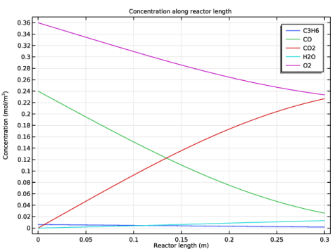
In the associated text field, type Reactor length (m).
|
|
5
|
|
1
|
|
2
|
|
3
|
|
1
|
|
2
|
|
3
|
|
4
|
Click
|
|
6
|
|
1
|
|
2
|
|
3
|
|
4
|
|
5
|
|
6
|
|
7
|
Click
|
|
1
|
|
2
|
|
1
|
|
2
|
|
3
|
|
4
|
|
5
|
|
6
|
|
7
|
|
8
|
|
9
|
|
10
|
|
1
|
|
2
|
|
3
|
|
4
|
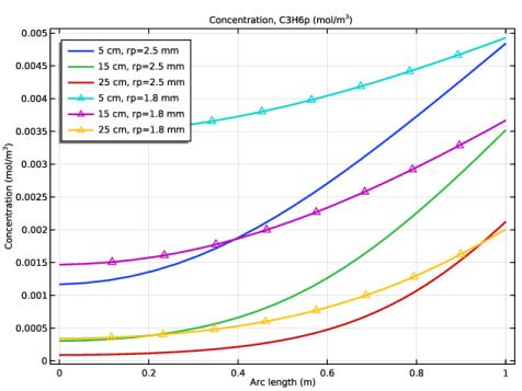
Locate the Coloring and Style section. Find the Line markers subsection. From the Marker list, choose Triangle.
|
|
1
|
|
2
|
|
3
|
|
4
|
|
5
|
|
6
|
|
1
|
|
2
|
|
3
|
|
4
|
|
5
|
In the associated text field, type Pressure (Pa).
|
|
6
|
|
1
|
|
2
|
|
3
|
|
4
|