PDF

Optimization of a Catalytic Microreactor
Introduction
In this model, a solution is pumped through a catalytic bed, where a reactant undergoes chemical reaction as it gets in contact with the catalyst. The purpose of the example is to maximize the total reaction rate for a given total pressure difference across the bed. This is achieved by finding an optimal catalyst distribution. The distribution of the porous catalyst determines the total reaction rate in the bed. A large amount of catalyst results in a low flow rate through the bed, while less catalyst gives a high flow rate but low conversion of the reactant.
This modeling example is based on Ref. 1.
Note: This application requires the Optimization Module.
Model Definition
The model geometry is shown in Figure 1. The reactor consists of an inlet channel, a fixed catalytic bed, and an outlet channel.
Figure 1: Model geometry.
The optimal catalyst distribution should maximize the average reaction rate, which is expressed as the integral of the local reaction rate, r (SI unit: mol/(m3·s)), over the domain, Ω. This is equivalent to minimizing the negative of this average reaction rate:
Assuming a first-order catalytic reaction with respect to the reactant species, the local reaction rate is determined by
(1)
where ε denotes the volume fraction of solid catalyst, c refers to the concentration (SI unit: mol/m3), and ka is the rate constant (SI unit: 1/s).
The mass transport is described by the convection and diffusion equation
where u denotes the velocity vector (SI unit: m/s) and D is the diffusion coefficient (SI unit: m2/s). The Navier-Stokes equations describe the fluid flow:
(2)
The coefficient α(ε) depends on the distribution of the porous catalyst as
(3)
where Da is the Darcy number; L is the length scale (SI unit: m); and q is a dimensionless parameter, the interpretation of which is discussed in the next section.
From Equation 3, the direct conclusion is that when ε equals 1, α equals zero and Equation 2 reduces to the ordinary Navier-Stokes equations. In this case the reaction rate is zero; see Equation 1.
To summarize, the optimization problem is
(4)
where
and physical boundary conditions apply.
Convex Optimization Problems
One of the most important characteristics of an optimization problem is whether or not the problem is convex. This section therefore briefly describes this property. For a more general discussion of the subject, see for example Ref. 2.
A set C is said to be convex if for any two members x, y of C, the following relation holds:
that is, the straight line between x and y is fully contained in C. A convex function is a mapping f from a convex set C such that for every two members x, y of C
(5)
An optimization problem is said to be convex if the following conditions are met:
The importance of convexity follows simply from the result that if x* is a local minimum to a convex optimization problem, then x* is also a global minimum. This is easily proven by simply assuming that there is a y such that f(y) < f(x*), and then using Equation 5.
This particular optimization problem is nonlinear, because a change in ε implies a change in the concentration, c. Because of this implicit dependence, it is very difficult to determine whether or not the objective is convex. There is therefore no guarantee that the optimal solution you obtain is globally optimal or unique. In the best of cases, running the optimization gives a good local optimum.
The parameter q can be used to smoothen the interfaces between the catalyst and the open channel. To see the effect of this parameter, rewrite Equation 3 as
It follows that when q approaches infinity, α is the (inverse) porosity. On the other hand, lowering the value of q decreases the magnitude of α.
Figure 2: q(1 − ε)/(q − ε) plotted as a function of ε for different values of q.
Figure 2 shows q(1 − ε)/(q − ε) plotted as a function of ε for different values of q. This plot shows that lowering the value of q, increases the convexity of the force coefficient. For a low q value, an increase in ε around 0.5, imposes a small increase of the force coefficient, while for a higher value of q, a change in ε imposes an almost equal change for the whole range. Therefore, for a lower q value, the solution is not sharp at the interfaces. On the other hand, for small values of ε, the force term decreases rapidly when q is small, and thus affects the flow field to a much wider extent. In the limit when q approaches infinity, α as a function of ε is a straight line.
Results and Discussion
Figure 3 shows the velocity field in the empty channel. This is the starting point for the optimization.
Figure 3: Velocity field in the open channel.
Figure 4: Distribution of the porous catalyst seen in black and open channel in white.
Figure 4 shows the distribution of the porous catalyst in black and the open channels in white. This result shows that, optimally, the supply of the reactant should be distributed over a large area of the reactor. Note also that the amount of open channel volume is significant.
Figure 5 shows the concentration distribution in the reactor. This plot shows how the porous catalyst is fed with the reactant through the open channels. The plot naturally resembles that of Figure 4.
Figure 5: Concentration distribution in the reactor after optimization.
Let
,
where nflow refers to the normal to the boundary ∂Ωi in the flow direction (that is, pointing in to the domain at the inlet and out from the domain at the outlet). Then Fi is a measurement of the flow of the species with concentration c through the boundary ∂Ωi per unit length in the transverse dimension. The conversion, X, of the reactant is defined as
In this case, the conversion of the reactant is around 50%.
Figure 6 shows the velocity field in the reactor. The porous catalyst slows down the flow significantly compared to Figure 3.
Figure 6: Velocity field in the reactor after optimization.
References
1. F. Okkels and H. Bruus, “Scaling Behavior of Optimally Structured Catalytic Microfluidic Reactors,” Phys. Rev. E, vol. 75, pp. 016301 1–4, 2007.
2. S.G. Nash and A. Sofer, Linear and Nonlinear Programming, McGraw-Hill, 1995.
Application Library path: Chemical_Reaction_Engineering_Module/Reactors_with_Mass_Transfer/microreactor_optimization
Modeling Instructions
From the File menu, choose New.
New
In the New window, click  Model Wizard.
Model Wizard
1
In the Model Wizard window, click  2D.
2
In the Select Physics tree, select Fluid Flow>Single-Phase Flow>Laminar Flow (spf).
3
Click Add.
4
In the Select Physics tree, select Chemical Species Transport>Transport of Diluted Species (tds).
5
Click Add.
6
Click  Study.
7
In the Select Study tree, select General Studies>Stationary.
8
Root
Load parameters from a text file.
Global Definitions
Parameters 1
1
In the Model Builder window, under Global Definitions click Parameters 1.
2
In the Settings window for Parameters, locate the Parameters section.
3
Click  Load from File.
4
Geometry 1
Next, create the geometry. The reactor consists of three domains: the inlet channel, the reacting domain, and the outlet channel (see Figure 1).
1
In the Model Builder window, under Component 1 (comp1) click Geometry 1.
2
In the Settings window for Geometry, locate the Units section.
3
From the Length unit list, choose mm.
Rectangle 1 (r1)
1
In the Geometry toolbar, click  Rectangle.
2
In the Settings window for Rectangle, locate the Size and Shape section.
3
In the Width text field, type 2*L.
4
In the Height text field, type L.
Rectangle 2 (r2)
1
In the Geometry toolbar, click  Rectangle.
2
In the Settings window for Rectangle, locate the Size and Shape section.
3
In the Width text field, type 6*L.
4
In the Height text field, type 3*L.
5
Locate the Position section. In the x text field, type 2*L.
6
Locate the Selections of Resulting Entities section. Select the Resulting objects selection check box.
Rectangle 3 (r3)
1
In the Geometry toolbar, click  Rectangle.
2
In the Settings window for Rectangle, locate the Size and Shape section.
3
In the Width text field, type 2*L.
4
In the Height text field, type L.
5
Locate the Position section. In the x text field, type 8*L.
6
Click  Build Selected.
7
Click the  Zoom Extents button in the Graphics toolbar.
The geometry should now look like that in Figure 1.
Define integration couplings to use for calculating the conversion of the reactant.
Definitions
Integration 1 (intop1)
1
In the Definitions toolbar, click  Nonlocal Couplings and choose Integration.
2
In the Settings window for Integration, locate the Source Selection section.
3
From the Geometric entity level list, choose Boundary.
4
Integration 2 (intop2)
1
In the Definitions toolbar, click  Nonlocal Couplings and choose Integration.
2
In the Settings window for Integration, locate the Source Selection section.
3
From the Geometric entity level list, choose Boundary.
4
Add a density topology feature, which can be used to distinguish between free flow and solid regions. This variable will be coupled back to the Laminar Flow interfaces later.
5
In the Definitions toolbar, click  Optimization and choose Topology Optimization>Density Model.
Topology Optimization
Density Model 1 (dtopo1)
Only the center part of the channel geometry is needed in the optimization, so you only have to define the feature there.
1
In the Settings window for Density Model, locate the Geometric Entity Selection section.
2
From the Selection list, choose Rectangle 2.
3
Locate the Filtering section. From the Filter type list, choose None.
4
Locate the Interpolation section. From the Interpolation type list, choose Darcy.
5
In the qDarcy text field, type q.
6
Locate the Control Variable Initial Value section. In the θ0 text field, type 1.
Now the design variable used in the optimization is defined. The initial value 1 corresponds to a channel free from porous material.
Definitions
Variables 1
1
In the Definitions toolbar, click  Local Variables.
Use the integration operators to define the conversion of reactant and the scaled objective function.
2
In the Settings window for Variables, locate the Variables section.
3
Here, tds.tfluxx_c is the COMSOL Multiphysics variable for the x-component of the total flux.
Variables 2
1
In the Definitions toolbar, click  Local Variables.
2
In the Settings window for Variables, locate the Geometric Entity Selection section.
3
From the Geometric entity level list, choose Domain.
4
5
Locate the Variables section. In the table, enter the following settings:
Objective Function
1
In the Definitions toolbar, click  Probes and choose Domain Probe.
2
In the Settings window for Domain Probe, type Objective Function in the Label text field.
3
In the Variable name text field, type obj.
4
Locate the Source Selection section. From the Selection list, choose Rectangle 2.
5
Click Replace Expression in the upper-right corner of the Expression section. From the menu, choose Component 1 (comp1)>Definitions>Variables>phi - Local reaction rate - mol/(m³·s).
Add Material
1
In the Home toolbar, click  Add Material to open the Add Material window.
2
Go to the Add Material window.
3
In the tree, select Built-in>Water, liquid.
4
Click Add to Component in the window toolbar.
5
In the Home toolbar, click  Add Material to close the Add Material window.
Laminar Flow (spf)
Volume Force 1
1
In the Model Builder window, under Component 1 (comp1) right-click Laminar Flow (spf) and choose Volume Force.
2
3
In the Settings window for Volume Force, locate the Volume Force section.
4
Specify the F vector as
Inlet 1
1
In the Physics toolbar, click  Boundaries and choose Inlet.
2
3
In the Settings window for Inlet, locate the Boundary Condition section.
4
5
Locate the Pressure Conditions section. In the p0 text field, type delta_p.
Symmetry 1
1
In the Physics toolbar, click  Boundaries and choose Symmetry.
2
Outlet 1
1
In the Physics toolbar, click  Boundaries and choose Outlet.
2
Transport of Diluted Species (tds)
Transport Properties 1
1
In the Model Builder window, under Component 1 (comp1)>Transport of Diluted Species (tds) click Transport Properties 1.
2
In the Settings window for Transport Properties, locate the Diffusion section.
3
In the Dc text field, type D.
Reactions 1
1
In the Physics toolbar, click  Domains and choose Reactions.
2
3
In the Settings window for Reactions, locate the Reaction Rates section.
4
In the Rc text field, type -phi.
Concentration 1
1
In the Physics toolbar, click  Boundaries and choose Concentration.
2
In the Settings window for Concentration, locate the Concentration section.
3
Select the Species c check box.
4
In the c0,c text field, type c_in.
5
Outflow 1
1
In the Physics toolbar, click  Boundaries and choose Outflow.
2
This example requires a fine mesh, both to solve the physics problem and to resolve the topology optimization problem.
Multiphysics
Couple the interfaces with the Reacting Flow multiphysics node.
Reacting Flow, Diluted Species 1 (rfd1)
In the Physics toolbar, click  Multiphysics Couplings and choose Domain>Reacting Flow, Diluted Species.
Mesh 1
1
In the Model Builder window, under Component 1 (comp1) click Mesh 1.
2
In the Settings window for Mesh, locate the Sequence Type section.
3
From the list, choose User-controlled mesh.
Size
1
In the Model Builder window, under Component 1 (comp1)>Mesh 1 click Size.
2
In the Settings window for Size, locate the Element Size section.
3
From the Calibrate for list, choose General physics.
4
From the Predefined list, choose Extremely fine.
Corner Refinement 1, Size 1
1
In the Model Builder window, under Component 1 (comp1)>Mesh 1, Ctrl-click to select Size 1 and Corner Refinement 1.
2
Boundary Layers 1
1
In the Model Builder window, right-click Boundary Layers 1 and choose Disable.
2
In the Settings window for Boundary Layers, click  Build All.
Study 1
Although you can choose to solve the optimization problem directly, it can be useful to check that the solution for the PDE problem looks sound before starting the optimization.
1
In the Home toolbar, click  Compute.
Results
Velocity (spf)
The first default plot (see Figure 3) shows the velocity field in the reactor.
Now solve the optimization problem.
Study 1
Topology Optimization
1
In the Study toolbar, click  Optimization and choose Topology Optimization.
2
In the Settings window for Topology Optimization, locate the Optimization Solver section.
3
In the Maximum number of iterations text field, type 50.
4
Click Add Expression in the upper-right corner of the Objective Function section. From the menu, choose Component 1 (comp1)>Definitions>comp1.obj - Objective Function - mol/(m³·s).
5
Locate the Objective Function section. From the Type list, choose Maximization.
6
From the Objective scaling list, choose Manual.
7
In the Scale text field, type 0.1.
8
Locate the Output While Solving section. Select the Plot check box.
This setting gives a plot of the evolving velocity distribution in the Graphics window.
Solution 1 (sol1)
1
In the Study toolbar, click  Show Default Solver.
The original MMA (1987) implementation has worse final convergence than GCMMA, but it can also be less prone to local minima, which is more important for many topology optimization problems.
2
In the Model Builder window, expand the Solution 1 (sol1) node, then click Optimization Solver 1.
3
In the Settings window for Optimization Solver, locate the Optimization Solver section.
4
Clear the Globally Convergent MMA check box.
5
Click to expand the Advanced section. From the Compensate for nojac terms list, choose Off to avoid warnings in the log.
6
In the Study toolbar, click  Compute.
Results
Velocity (spf)
The velocity field in the reactor after optimization should resemble that in Figure 6.
Concentration (tds)
The third default plot shows the concentration distribution in the reactor after optimization (Figure 5).
Streamline 1
1
In the Model Builder window, expand the Concentration (tds) node, then click Streamline 1.
2
In the Settings window for Streamline, locate the Streamline Positioning section.
3
From the Positioning list, choose On selected boundaries.
4
In the Number text field, type 5.
5
Locate the Selection section. Click to select the  Activate Selection toggle button.
6
7
In the Concentration (tds) toolbar, click  Plot.
To reproduce the plot in Figure 4, modify the default plot with the following steps.
Distribution of porous catalyst
1
In the Model Builder window, expand the Results>Topology Optimization node, then click Output material volume factor.
2
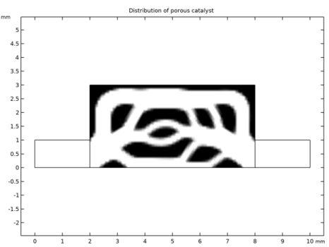
In the Settings window for 2D Plot Group, type Distribution of porous catalyst in the Label text field.
3
Click to expand the Title section. From the Title type list, choose Manual.
4
In the Title text area, type Distribution of porous catalyst.
Surface 1
1
In the Model Builder window, expand the Distribution of porous catalyst node, then click Surface 1.
2
In the Settings window for Surface, locate the Coloring and Style section.
3
From the Color table list, choose GrayScale.
4
Clear the Color legend check box.
5
In the Distribution of porous catalyst toolbar, click  Plot.
6
Click the  Zoom Extents button in the Graphics toolbar.
To display the result for the conversion rate, continue as follows.
Global Evaluation 1
1
In the Results toolbar, click  Global Evaluation.
2
In the Settings window for Global Evaluation, click Add Expression in the upper-right corner of the Expressions section. From the menu, choose Solver>Objective functions>opt.obj1 - Objective Function - mol/(m³·s).
3
Click  Evaluate.
Table
1
Go to the Table window.
The value appears in the Table window below the Graphics window.