PDF

Microchannel H-Cell
Introduction
This example models an H-microcell for separation through diffusion. In Figure 1, it is shown how the cell puts two different laminar streams in contact for a controlled period of time. The contact surface is well defined, and by controlling the flow rate it is possible to control the amount of species transported from one stream to the other through diffusion. This example was originally formulated by Albert Witarsa under Professor Bruce Finlayson’s supervision at the University of Washington in Seattle. It was part of a graduate course in which the assignment consisted of using mathematical modeling to evaluate the potential of patents in the field of microfluidics.
The model utilizes the Laminar Flow and Transport of Diluted Species interfaces to fully capture the separation within the cell.
Figure 1: Diagram of the H-microcell (dimensions in meters).
Model Definition
The geometry of the microcell is shown in Figure 2. Due to symmetry, the model geometry can be simplified to half of it.
The design is aimed to eliminate upsets in the flow field when the two streams, A and B, are united. Thus, the cell enables mixing of A and B solely through diffusion. A system allowing convection would mix all species equally and lead to loss of control over the separation abilities.
Figure 2: Model geometry as given by Albert Witarsa’s and Professor Finlayson. To avoid any type of convective mixing, the design must smoothly let both streams come in contact with each other. Due to symmetry, it is sufficient to model half the geometry.
The simulations involve solving the fluid flow in the H-cell. According to the specifications, the flow rate at the inlet is roughly 0.1 mm/s. This implies a low Reynolds number, well inside the region of laminar flow:
(1)
Equation 1 gives a Reynolds number of 0.001 for a water solution and the channel dimensions given in Figure 1. This value is typical for microchannels. Additionally, this indicates that it is easy to get a numerical solution of the full momentum balance and continuity equations with a reasonable number of elements. The Laminar Flow interface can set up and solve the incompressible Navier-Stokes equations at steady state:
Here ρ denotes density (SI unit: kg/m3), u is the velocity (SI unit: m/s), μ denotes viscosity (SI unit: Pa·s), and p equals pressure (SI unit: Pa).
Separation in the H-cell involves species in relatively low concentrations compared to the solvent, in this case water. This means that the solute molecules interact only with water molecules, and it is safe to use Fick’s law to describe the diffusive transport in the cell. Use the Transport of Diluted Species interface to set up and solve the appropriate stationary mass-balance equation:
(2)
In this equation, D denotes the diffusion coefficient (SI unit: m2/s) and c represents the concentration (SI unit: mol/m3). In this model, you use the parametric solver to solve Equation 2 for three different values of D1·1011 m2/s, 5·1011 m2/s, and 1·1010 m2/s —  to simulate the mixing of different species.
You solve two versions of the model:
(3)
Here α is a constant of dimension (SI unit: m6/mol2). An influence of concentration on viscosity of this kind is usually observed in solutions of larger molecules. In this case the flow and mass transport equations have to be solved simultaneously.
Last, consider the boundary conditions. All boundaries are visualized in Figure 3.
Figure 3: Model domain boundaries.
For the Laminar Flow interface:
For the Transport of Diluted Species:
Results and Discussion
Figure 4 shows the velocity field for the whole microcell. The flow is symmetric and is not influenced by the concentration field.
Figure 4: Flow velocity field.
Figure 5 shows the concentration distribution for the species with the highest simulated diffusivity.
Figure 5: Concentration distribution for a species with diffusivity 1010 m2/s.
Because of the relatively large diffusion coefficient, the degree of mixing is almost perfect. The species with a diffusion coefficient ten times smaller shows a different result. The concentration distribution in Figure 6 shows that the diffusion coefficient for the species too low for achieving significant mixing of the streams.
Figure 6: Concentration distribution for a species with diffusivity 1·1011m2/s.
The simulation clearly shows that the H-cell can separate lighter molecules from heavier ones. A cascade of H-cells can achieve a very high degree of separation.
In some cases, especially those involving solutions of macromolecules, the macromolecule concentration has a large influence on the liquid’s viscosity. In such situations, the model needs to be fully coupled and solve both interfaces simultaneously. Figure 7 shows the results of such a simulation. Here, the changes in viscosity have caused an asymmetry in the velocity. As a consequence of the modified flow field, the transport of molecules to outlet B is also different from the constant flow field case (Figure 8 versus Figure 5).
Figure 7: Velocity field. The viscosity varies with the concentration according to Equation 3 with α = 0.5 (m3/mol)2. The figure shows that the velocity field is affected by variations in concentration..
Figure 8: Concentration distribution for the species with diffusivity 1·1010m2/s for the case where the fluid viscosity varies with concentration. Comparison with the plot in Figure 5 shows that fewer molecules of the species are transported to outlet B.
Application Library path: Chemical_Reaction_Engineering_Module/Mixing_and_Separation/microchannel_h_cell
Modeling Instructions
From the File menu, choose New.
New
In the New window, click  Model Wizard.
Model Wizard
1
In the Model Wizard window, click  3D.
2
In the Select Physics tree, select Fluid Flow>Single-Phase Flow>Laminar Flow (spf).
3
Click Add.
4
In the Select Physics tree, select Chemical Species Transport>Transport of Diluted Species (tds).
5
Click Add.
6
Click  Study.
7
In the Select Study tree, select General Studies>Stationary.
8
Geometry 1
Create the geometry. To simplify this step, insert a prepared geometry sequence.
1
In the Model Builder window, under Component 1 (comp1) click Geometry 1.
2
In the Geometry toolbar, click Insert Sequence.
3
Work Plane 1 (wp1)
1
Click the  Zoom Extents button in the Graphics toolbar.
This completes the geometry modeling stage. The geometry should now look like that in the figure below.
Root
Import the model parameters from a text file.
Global Definitions
Parameters 1
1
In the Model Builder window, under Global Definitions click Parameters 1.
2
In the Settings window for Parameters, locate the Parameters section.
3
Click  Load from File.
4
The material properties of water are available within the Material Library.
Add Material
1
In the Home toolbar, click  Add Material to open the Add Material window.
2
Go to the Add Material window.
3
In the tree, select Built-in>Water, liquid.
4
Click Add to Component in the window toolbar.
5
In the Home toolbar, click  Add Material to close the Add Material window.
For microfluidic flows, second order elements are more accurate and computationally efficient than the linear elements. Increase the element order for both interfaces in the model.
Laminar Flow (spf)
1
In the Model Builder window, under Component 1 (comp1) click Laminar Flow (spf).
2
In the Settings window for Laminar Flow, click to expand the Discretization section.
3
From the Discretization of fluids list, choose P2+P1.
Transport of Diluted Species (tds)
1
In the Model Builder window, under Component 1 (comp1) click Transport of Diluted Species (tds).
2
In the Settings window for Transport of Diluted Species, click to expand the Discretization section.
3
From the Concentration list, choose Quadratic.
Laminar Flow (spf)
In the Model Builder window, under Component 1 (comp1) click Laminar Flow (spf).
Inlet 1
1
In the Physics toolbar, click  Boundaries and choose Inlet.
2
3
In the Settings window for Inlet, locate the Boundary Condition section.
4
5
Locate the Pressure Conditions section. In the p0 text field, type p0.
Outlet 1
1
In the Physics toolbar, click  Boundaries and choose Outlet.
2
3
In the Settings window for Outlet, locate the Pressure Conditions section.
4
Select the Normal flow check box.
Symmetry 1
1
In the Physics toolbar, click  Boundaries and choose Symmetry.
2
Transport of Diluted Species (tds)
Transport Properties 1
1
In the Model Builder window, under Component 1 (comp1)>Transport of Diluted Species (tds) click Transport Properties 1.
2
In the Settings window for Transport Properties, locate the Diffusion section.
3
In the Dc text field, type D.
Concentration 1
1
In the Physics toolbar, click  Boundaries and choose Concentration.
2
3
In the Settings window for Concentration, locate the Concentration section.
4
Select the Species c check box.
5
In the c0,c text field, type c0.
Concentration 2
1
In the Physics toolbar, click  Boundaries and choose Concentration.
2
3
In the Settings window for Concentration, locate the Concentration section.
4
Select the Species c check box.
Outflow 1
1
In the Physics toolbar, click  Boundaries and choose Outflow.
2
Multiphysics
Reacting Flow, Diluted Species 1 (rfd1)
In the Physics toolbar, click  Multiphysics Couplings and choose Domain>Reacting Flow, Diluted Species.
Mesh 1
1
In the Model Builder window, under Component 1 (comp1) click Mesh 1.
2
In the Settings window for Mesh, locate the Physics-Controlled Mesh section.
3
From the Element size list, choose Coarse.
Size
Right-click Component 1 (comp1)>Mesh 1 and choose Edit Physics-Induced Sequence.
Size 1
1
In the Settings window for Size, locate the Element Size section.
2
From the Predefined list, choose Coarser.
3
Click  Build Selected.
Size 2
1
In the Model Builder window, right-click Mesh 1 and choose Size.
2
In the Settings window for Size, locate the Geometric Entity Selection section.
3
From the Geometric entity level list, choose Point.
4
5
Locate the Element Size section. Click the Custom button.
6
Locate the Element Size Parameters section. Select the Maximum element size check box.
7
Free Tetrahedral 1
1
In the Model Builder window, right-click Free Tetrahedral 1 and choose Build Selected.
2
In the Settings window for Free Tetrahedral, click  Build All.
Use two Stationary solver steps. In the first only the Laminar Flow interface is solved.
Study 1
Step 1: Stationary
1
In the Model Builder window, under Study 1 click Step 1: Stationary.
2
In the Settings window for Stationary, locate the Physics and Variables Selection section.
3
In the table, clear the Solve for check box for Transport of Diluted Species (tds).
Add a second stationary step that solves the Transport of Diluted Species interface using the previously computed flow field.
Stationary 2
1
In the Study toolbar, click  Study Steps and choose Stationary>Stationary.
2
In the Settings window for Stationary, locate the Physics and Variables Selection section.
3
In the table, clear the Solve for check box for Laminar Flow (spf).
Within this study step, enable the parametric continuation solver to solve the mass transport problem for several diffusion coefficients.
4
Click to expand the Study Extensions section. Select the Auxiliary sweep check box.
5
6
Solution 1 (sol1)
1
In the Study toolbar, click  Show Default Solver.
By default, the solution from the first step will be applied to the (fluid) variables not solved for in the second step.
2
In the Settings window for Solution, click  Compute.
Create a Mirror 3D dataset that enables plotting of the whole geometry, that is, both sides of the symmetry plane.
Results
Mirror 3D 1
1
In the Results toolbar, click  More Datasets and choose Mirror 3D.
2
In the Settings window for Mirror 3D, locate the Plane Data section.
3
From the Plane list, choose xy-planes.
4
In the z-coordinate text field, type 1e-5.
Velocity (spf)
To generate Figure 4 follow these steps:
Slice
1
In the Model Builder window, expand the Velocity (spf) node, then click Slice.
2
In the Settings window for Slice, locate the Expression section.
3
From the Unit list, choose mm/s.
4
In the Velocity (spf) toolbar, click  Plot.
Slice 2
1
Right-click Slice and choose Duplicate.
2
In the Settings window for Slice, click to expand the Title section.
3
From the Title type list, choose None.
4
Locate the Plane Data section. From the Plane list, choose zx-planes.
5
In the Planes text field, type 2.
6
Click to expand the Inherit Style section. From the Plot list, choose Slice.
7
In the Velocity (spf) toolbar, click  Plot.
Slice 3
1
Right-click Slice 2 and choose Duplicate.
2
In the Settings window for Slice, locate the Plane Data section.
3
From the Plane list, choose xy-planes.
4
In the Planes text field, type 1.
5
From the Entry method list, choose Coordinates.
6
In the z-coordinates text field, type 1e-5.
7
In the Velocity (spf) toolbar, click  Plot.
Arrow Volume 1
1
In the Model Builder window, right-click Velocity (spf) and choose Arrow Volume.
2
In the Settings window for Arrow Volume, locate the Arrow Positioning section.
3
Find the x grid points subsection. In the Points text field, type 14.
4
Find the y grid points subsection. In the Points text field, type 21.
5
Find the z grid points subsection. In the Points text field, type 3.
6
Locate the Coloring and Style section. From the Color list, choose Black.
7
In the Velocity (spf) toolbar, click  Plot.
Velocity (spf)
1
In the Model Builder window, click Velocity (spf).
2
In the Settings window for 3D Plot Group, locate the Data section.
3
From the Dataset list, choose Mirror 3D 1.
4
Locate the Plot Settings section. From the Color list, choose Gray.
5
Click the  Show Grid button in the Graphics toolbar.
Slice
1
In the Model Builder window, click Slice.
2
In the Settings window for Slice, locate the Expression section.
3
From the Unit list, choose m/s.
4
Click to expand the Quality section. From the Resolution list, choose Fine.
5
Locate the Coloring and Style section. From the Color table list, choose RainbowLight.
Slice 2
1
In the Model Builder window, click Slice 2.
2
In the Settings window for Slice, locate the Expression section.
3
From the Unit list, choose m/s.
Slice 3
1
In the Model Builder window, click Slice 3.
2
In the Settings window for Slice, locate the Expression section.
3
From the Unit list, choose m/s.
Color Expression 1
1
In the Model Builder window, right-click Arrow Volume 1 and choose Color Expression.
2
In the Settings window for Color Expression, locate the Coloring and Style section.
3
From the Color table list, choose RainbowLight.
Arrow Volume 1
1
In the Model Builder window, click Arrow Volume 1.
2
In the Settings window for Arrow Volume, locate the Coloring and Style section.
3
Select the Scale factor check box.
4
5
Click to expand the Inherit Style section. From the Plot list, choose Slice.
6
In the Velocity (spf) toolbar, click  Plot.
7
Click the  Zoom Extents button in the Graphics toolbar.
8
In the Velocity (spf) toolbar, click  Plot.
Proceed to plot the concentration distribution Figure 5.
Concentration, Slice
1
In the Home toolbar, click  Add Plot Group and choose 3D Plot Group.
2
In the Settings window for 3D Plot Group, type Concentration, Slice in the Label text field.
3
Locate the Data section. From the Dataset list, choose Mirror 3D 1.
4
From the Parameter value (D (m^2/s)) list, choose 1E-10.
Slice 1
1
Right-click Concentration, Slice and choose Slice.
2
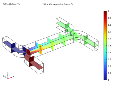
In the Settings window for Slice, click Replace Expression in the upper-right corner of the Expression section. From the menu, choose Component 1 (comp1)>Transport of Diluted Species>Species c>c - Concentration - mol/m³.
Slice 2
1
Right-click Slice 1 and choose Duplicate.
2
In the Settings window for Slice, locate the Title section.
3
From the Title type list, choose None.
4
Locate the Plane Data section. From the Plane list, choose zx-planes.
5
In the Planes text field, type 2.
6
Locate the Inherit Style section. From the Plot list, choose Slice 1.
7
In the Concentration, Slice toolbar, click  Plot.
Slice 3
1
Right-click Slice 2 and choose Duplicate.
2
In the Settings window for Slice, locate the Plane Data section.
3
From the Plane list, choose xy-planes.
4
In the Planes text field, type 1.
5
From the Entry method list, choose Coordinates.
6
In the z-coordinates text field, type 1e-5.
7
Click the  Zoom Extents button in the Graphics toolbar.
8
In the Concentration, Slice toolbar, click  Plot.
Concentration, Slice
Generate Figure 6 using the diffusion coefficient value 1E11 m2/s.
1
In the Model Builder window, click Concentration, Slice.
2
In the Settings window for 3D Plot Group, locate the Data section.
3
From the Parameter value (D (m^2/s)) list, choose 1E-11.
4
Click the  Zoom Extents button in the Graphics toolbar.
5
In the Concentration, Slice toolbar, click  Plot.
Add a correction term in the viscosity.
Laminar Flow (spf)
Fluid Properties 1
1
In the Model Builder window, under Component 1 (comp1)>Laminar Flow (spf) click Fluid Properties 1.
2
In the Settings window for Fluid Properties, locate the Fluid Properties section.
3
From the μ list, choose User defined. In the associated text field, type mu*(1+alpha*c^2).
When viscosity is concentration dependent you must solve all equations simultaneously. Add a second study for the fully coupled problem.
Add Study
1
In the Home toolbar, click  Add Study to open the Add Study window.
2
Go to the Add Study window.
3
Find the Studies subsection. In the Select Study tree, select General Studies>Stationary.
4
Click Add Study in the window toolbar.
5
In the Home toolbar, click  Add Study to close the Add Study window.
Study 2
1
In the Model Builder window, click Study 2.
2
In the Settings window for Study, locate the Study Settings section.
3
Clear the Generate default plots check box.
4
In the Home toolbar, click  Compute.
Create Figure 7 and Figure 8 by following these steps.
Results
Mirror 3D 2
1
In the Results toolbar, click  More Datasets and choose Mirror 3D.
2
In the Settings window for Mirror 3D, locate the Plane Data section.
3
From the Plane list, choose xy-planes.
4
In the z-coordinate text field, type 1e-5.
5
Locate the Data section. From the Dataset list, choose Study 2/Solution 3 (sol3).
Velocity (spf) 1
1
In the Model Builder window, right-click Velocity (spf) and choose Duplicate.
2
In the Settings window for 3D Plot Group, locate the Data section.
3
From the Dataset list, choose Mirror 3D 2.
4
Click the  Zoom Extents button in the Graphics toolbar.
5
In the Velocity (spf) 1 toolbar, click  Plot.
6
Click the  Show Grid button in the Graphics toolbar.
Concentration, Slice 1
1
In the Model Builder window, right-click Concentration, Slice and choose Duplicate.
2
In the Settings window for 3D Plot Group, locate the Data section.
3
From the Dataset list, choose Mirror 3D 2.
4
Click the  Zoom Extents button in the Graphics toolbar.
5
In the Concentration, Slice 1 toolbar, click  Plot.
6
Click the  Show Grid button in the Graphics toolbar.