|
|
|
|
1
|
|
2
|
In the Select Physics tree, select Fluid Flow>Nonisothermal Flow>Turbulent Flow>Turbulent Flow, k-ε.
|
|
3
|
Click Add.
|
|
4
|
Click
|
|
5
|
|
6
|
Click
|
|
1
|
|
2
|
|
3
|
Click Next in the window toolbar.
|
|
1
|
|
2
|
|
3
|
|
4
|
|
5
|
|
6
|
|
7
|
Click Next in the window toolbar.
|
|
1
|
|
2
|
|
3
|
Click Finish in the window toolbar.
|
|
1
|
In the Model Builder window, under Global Definitions>Thermodynamics right-click Vapor-Liquid System 1 (pp1) and choose Generate Material.
|
|
1
|
|
2
|
From the list, choose Liquid.
|
|
3
|
Click Next in the window toolbar.
|
|
1
|
|
2
|
|
3
|
Click Next in the window toolbar.
|
|
1
|
|
2
|
Click Next in the window toolbar.
|
|
1
|
|
2
|
Click Finish in the window toolbar.
|
|
1
|
|
2
|
|
3
|
|
4
|
Browse to the model’s Application Libraries folder and double-click the file engine_coolant_properties_parameters.txt.
|
|
1
|
|
2
|
|
3
|
|
4
|
|
5
|
|
6
|
|
1
|
|
2
|
|
3
|
|
4
|
|
5
|
|
6
|
|
1
|
|
2
|
|
3
|
|
4
|
|
5
|
|
6
|
|
1
|
|
2
|
|
3
|
|
4
|
|
5
|
|
6
|
|
1
|
|
2
|
|
3
|
|
4
|
|
5
|
|
1
|
|
2
|
|
3
|
|
4
|
|
5
|
|
1
|
|
2
|
On the object uni1, select Point 5 only.
|
|
3
|
On the object uni2, select Points 6, 7, 9, and 10 only.
|
|
4
|
|
5
|
|
6
|
|
1
|
|
2
|
In the Settings window for Study, type Study 1: Mixture properties parameterization in the Label text field.
|
|
3
|
|
1
|
In the Model Builder window, under Study 1: Mixture properties parameterization click Step 1: Stationary.
|
|
2
|
|
3
|
|
4
|
Click
|
|
6
|
|
7
|
Locate the Physics and Variables Selection section. In the table, clear the Solve for check boxes for Turbulent Flow, k-ε (spf) and Heat Transfer in Fluids (ht).
|
|
8
|
|
9
|
|
1
|
|
2
|
|
3
|
|
1
|
|
2
|
In the Settings window for Global, click Replace Expression in the upper-right corner of the y-Axis Data section. From the menu, choose Global definitions>Functions>Densitypp1(temperature, pressure, massfraction_ethylene_glycol, massfraction_water) - Density 1.
|
|
3
|
|
4
|
|
1
|
|
2
|
|
3
|
|
4
|
|
5
|
|
6
|
|
7
|
|
1
|
|
2
|
|
3
|
|
1
|
|
2
|
In the Settings window for Global, click Replace Expression in the upper-right corner of the y-Axis Data section. From the menu, choose Global definitions>Functions>Viscositypp1(temperature, pressure, massfraction_ethylene_glycol, massfraction_water) - Viscosity 1.
|
|
3
|
|
4
|
|
1
|
|
2
|
|
3
|
|
4
|
|
5
|
|
6
|
|
7
|
|
1
|
|
2
|
|
3
|
|
1
|
|
2
|
In the Settings window for Global, click Replace Expression in the upper-right corner of the y-Axis Data section. From the menu, choose Global definitions>Functions>ThermalConductivitypp1(temperature, pressure, massfraction_ethylene_glycol, massfraction_water) - Thermal conductivity 1.
|
|
3
|
|
4
|
|
1
|
|
2
|
|
3
|
|
4
|
In the associated text field, type Temperature (K).
|
|
5
|
|
6
|
In the associated text field, type Thermal conductivity (W/(m*K)).
|
|
7
|
|
8
|
|
1
|
|
2
|
|
3
|
|
1
|
|
2
|
In the Settings window for Global, click Replace Expression in the upper-right corner of the y-Axis Data section. From the menu, choose Global definitions>Functions>HeatCapacityCppp1(temperature, pressure, massfraction_ethylene_glycol, massfraction_water) - Heat capacity (Cp) 1.
|
|
3
|
|
4
|
|
1
|
|
2
|
|
3
|
|
4
|
In the associated text field, type Temperature (K).
|
|
5
|
|
6
|
In the associated text field, type Heat capacity (J/(kg*K)).
|
|
7
|
|
8
|
|
1
|
|
2
|
|
3
|
Click Next in the window toolbar.
|
|
1
|
|
2
|
|
3
|
|
4
|
|
5
|
Click Next in the window toolbar.
|
|
1
|
|
2
|
Click Finish in the window toolbar.
|
|
1
|
|
2
|
|
3
|
|
4
|
Locate the Definition section. In the Expression text field, type Flash1_1_Temperature(p,n,w_EG,w_W).
|
|
5
|
|
6
|
Locate the Units section. In the table, enter the following settings:
|
|
7
|
|
1
|
|
2
|
|
3
|
|
4
|
|
5
|
|
1
|
|
2
|
|
3
|
Click
|
|
5
|
|
6
|
|
7
|
In the Settings window for Study, type Study 2: Phase envelope parameterization in the Label text field.
|
|
8
|
|
9
|
|
10
|
|
11
|
In the table, clear the Solve for check boxes for Turbulent Flow, k-ε (spf) and Heat Transfer in Fluids (ht).
|
|
12
|
|
13
|
|
1
|
|
2
|
|
3
|
|
4
|
|
5
|
|
6
|
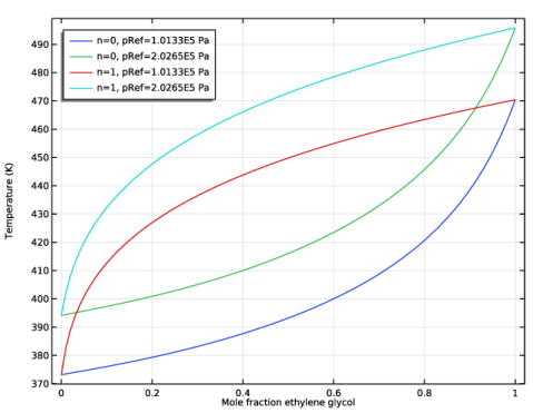
In the associated text field, type Mole fraction ethylene glycol.
|
|
7
|
|
8
|
In the associated text field, type Temperature (K).
|
|
1
|
|
2
|
|
4
|
|
5
|
|
1
|
|
2
|
|
3
|
|
4
|
|
5
|
|
6
|
Click OK.
|
|
1
|
In the Model Builder window, expand the Component 1 (comp1)>Materials node, then click Liquid: ethylene glycol-water 1 (pp1mat1).
|
|
3
|
|
4
|
|
1
|
|
1
|
|
3
|
|
4
|
|
1
|
|
1
|
|
3
|
|
4
|
|
5
|
|
6
|
|
1
|
|
1
|
|
3
|
|
4
|
|
5
|
|
1
|
|
1
|
|
2
|
|
3
|
|
4
|
|
5
|
|
1
|
|
2
|
|
3
|
|
4
|
Find the Physics interfaces in study subsection. In the table, clear the Solve check box for Heat Transfer in Fluids (ht).
|
|
5
|
|
1
|
|
2
|
|
3
|
Click
|
|
5
|
|
6
|
|
1
|
|
2
|
|
3
|
|
4
|
Click
|
|
1
|
|
2
|
|
3
|
In the Model Builder window, expand the Study 3: Water>Solver Configurations>Solution 3 (sol3)>Stationary Solver 2 node, then click Segregated 1.
|
|
4
|
|
5
|
|
6
|
|
1
|
In the Model Builder window, under Results, Ctrl-click to select Velocity (spf), Pressure (spf), Temperature, 3D (ht), and Isothermal Contours (ht).
|
|
2
|
Right-click and choose Delete.
|
|
1
|
|
2
|
|
3
|
|
1
|
|
2
|
|
3
|
|
4
|
|
5
|
|
6
|
|
7
|
|
8
|
|
1
|
|
2
|
|
3
|
|
4
|
|
5
|
|
6
|
|
7
|
|
8
|
In the associated text field, type Temperature (K).
|
|
1
|
|
2
|
|
3
|
|
4
|
|
5
|
|
1
|
|
2
|
|
3
|
Click
|
|
1
|
|
2
|
|
1
|
|
2
|
|
3
|
Find the Initial values of variables solved for subsection. From the Settings list, choose User controlled.
|
|
4
|
|
5
|
|
1
|
|
2
|
|
3
|
In the Model Builder window, expand the Study 4>Solver Configurations>Solution 5 (sol5)>Stationary Solver 1 node, then click Segregated 1.
|
|
4
|
|
5
|
|
6
|
In the Model Builder window, collapse the Study 4>Solver Configurations>Solution 5 (sol5)>Stationary Solver 1 node.
|
|
7
|
In the Model Builder window, expand the Study 4>Solver Configurations>Solution 5 (sol5)>Stationary Solver 2 node, then click Segregated 1.
|
|
8
|
|
9
|
|
10
|
|
11
|
|
12
|
|
13
|
|
14
|
In the Model Builder window, under Study 4: Glycol and Water>Solver Configurations>Solution 5 (sol5) click Solution Store 2 (sol6).
|
|
15
|
|
16
|
|
17
|
|
1
|
|
2
|
|
3
|
|
4
|
|
5
|
|
6
|
|
1
|
|
2
|
|
3
|
|
4
|
|
5
|
|
6
|
|
1
|
|
2
|
|
3
|
|
1
|
|
2
|
|
3
|
|
1
|
|
2
|
|
3
|
|
4
|
|
5
|
|
6
|
|
7
|
|
9
|
|
1
|
|
2
|
|
3
|
|
4
|
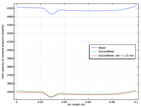
Locate the Legends section. In the table, enter the following settings:
|
|
5
|
|
1
|
|
2
|
|
3
|
|
4
|
Locate the Legends section. In the table, enter the following settings:
|
|
5
|
|
1
|
|
2
|
|
3
|
|
4
|
|
5
|
|
6
|
In the Rename 1D Plot Group dialog box, type Heat Capacity, Chamber Cut Line in the New label text field.
|
|
7
|
Click OK.
|
|
1
|
|
2
|
|
3
|
|
5
|
Locate the Expressions section. In the table, enter the following settings:
|
|
6
|
Click
|
|
1
|
|
2
|
|
1
|
|
2
|
|
3
|
|
4
|
|
5
|
|
6
|
|
1
|
In the Model Builder window, under Component 1 (comp1)>Turbulent Flow, k-ε (spf) click Fluid Properties 1.
|
|
2
|
|
3
|
|
1
|
|
2
|
|
3
|
|
4
|
|
5
|
|
1
|
|
2
|
Find the Initial values of variables solved for subsection. From the Settings list, choose User controlled.
|
|
3
|
|
4
|
|
5
|
|
6
|
In the Settings window for Study, type Study 5: Glycol and Water, Constant Properties in the Label text field.
|
|
7
|
|
8
|
|
1
|
|
2
|
|
3
|
|
4
|
|
1
|
|
3
|
|
5
|
|
6
|
Click
|
|
7
|
|
8
|
|
9
|
|
10
|
|
11
|
|
12
|
|
1
|
|
3
|
|
5
|
|
6
|
|
7
|
|
8
|
|
9
|
|
10
|
|
11
|
|
12
|
|
1
|
|
3
|
|
5
|
|
6
|
|
7
|
|
8
|
|
9
|
|
10
|
|
11
|
|
12
|