PDF

Neutralization of Chlorine in a Scrubber
Introduction
This application studies the kinetics of the neutralization of chlorine gas in water solution. It assumes that the fluid volume is perfectly mixed and constant. This means that the chlorine has dissolved to an almost saturated state (1 × 102 mol/m3) and that the hydroxide has also mixed well throughout, as would be the case for a very small amount of fluid in a scrubber. The study allows investigation of the time-scale of the reactions and the concentrations of the resulting products. A study of this type can be useful to determine the amount of hydroxide required to neutralize the chlorine and for sizing of a chlorine scrubber.
The example illustrates the functionality of the Reaction Engineering interface available in the Chemical Reaction Engineering Module to study chemical processes involving several equilibrium reactions.
Model Definition
The model includes four equilibrium reactions that take place in a constant volume batch reactor.
Chlorine neutralization by hydroxide ions:
(1)
Autoionization of water:
(2)
Formed hypochlorous acid reacting with hydroxide ions:
(3)
Chlorine reaction with water:
(4)
Traditionally, when setting up the reaction terms and mass balances of a reaction scheme, a full description of the mass action law is required. This includes reaction rate constants for both the forward and reverse reactions in the reaction term and subsequent mass balances. In the present example, you can assume that the forward and reverse reaction rate constants for Equation 2 and Equation 3 are not available, and that you have to use equilibrium constants instead. This is easily achieved using the Reaction Engineering interface.
The thermodynamic and kinetic data for the system are found in Ref. 1 and Ref. 2. These are listed in Table 1 below.
kf 
kr 
Keq
There are eight species participates in the reactions, of which one — H2O is the solvent. The parameters in Table 1 are valid for a solvent concentration set to unity. The only other non-vanishing initial concentration is that for chlorine in water, which is set to the value of 1·102 mol/m3. Yet, it is always useful to avoid zero concentrations throughout a specified reaction model, because they often show up in the participating equations, such as in those describing equilibrium. Therefore, some arbitrary trace concentrations are entered for the other species.
Results
Figure 1 shows the concentration profile during the first second of reaction.
Figure 1: Dissolved chlorine (aq), hydrogen ion, and hydroxide ion concentration in a log scale versus logarithmic time graph.
Initially, the chlorine quickly decays through the ready abundance of hydroxide ions. It continues to be reduced at a slower pace through the reaction with hydroxide ions that are, in turn, being produced through the water dissociation reaction. The initial concentration of the hydroxide ions is sufficiently large to guarantee an alkaline final solution.
A basic conclusion that can be drawn from this figure, is that a contact time of at least 150 ms is required to reduce the chlorine concentration to levels below 106 mol/m3. This is quite a short time in comparison with, for example, the time scale associated with the transport of chlorine into water.
References
1. C.W. Spalding, “Reaction Kinetics in the Absorption of Chlorine into Aqueous Media,” AIChE J., vol. 8, no. 5, pp. 685–689, 1962.
2. S.S. Ashour, E.B. Rinker, and O.C. Sandall, Absorption of Chlorine into Aqueous Bicarbonate Solutions and Aqueous Hydroxide Solutions, AIChE J., 42, 671, 1996.
Application Library path: Chemical_Reaction_Engineering_Module/Ideal_Tank_Reactors/chlorine_scrubber
Modeling Instructions
From the File menu, choose New.
New
In the New window, click  Model Wizard.
Model Wizard
1
In the Model Wizard window, The model utilizes the Reaction Engineering interface with a time-dependent study.
2
3
In the Select Physics tree, select Chemical Species Transport>Reaction Engineering (re).
4
Click Add.
5
Click  Study.
6
In the Select Study tree, select General Studies>Time Dependent.
7
Global Definitions
Start by reading in a set of global parameters.
Parameters 1
1
In the Model Builder window, under Global Definitions click Parameters 1.
2
In the Settings window for Parameters, locate the Parameters section.
3
Click  Load from File.
4
The default reactor type, Batch, constant volume, is used in this study. The reactions are studied for isothermal condition.
Reaction Engineering (re)
1
In the Model Builder window, under Component 1 (comp1) click Reaction Engineering (re).
2
In the Settings window for Reaction Engineering, locate the Energy Balance section.
3
In the T text field, type Temp.
4
Click to expand the Mixture Properties section. From the Phase list, choose Liquid.
Set up each of the equilibrium reactions and enter the reaction properties. Use the default reaction rate expressions.
Reaction 1
1
In the Reaction Engineering toolbar, click  Reaction.
2
In the Settings window for Reaction, locate the Reaction Formula section.
3
In the Formula text field, type Cl2+OH<=>HClO+Cl.
4
Click Apply.
5
Locate the Rate Constants section. In the kf text field, type kfreac_1.
6
In the kr text field, type krreac_1.
Reaction 2
1
In the Reaction Engineering toolbar, click  Reaction.
2
In the Settings window for Reaction, locate the Reaction Formula section.
3
In the Formula text field, type H+OH=H2O.
4
Click Apply.
5
Locate the Equilibrium Settings section. In the Keq0 text field, type Kequi_2.
Reaction 3
1
In the Reaction Engineering toolbar, click  Reaction.
2
In the Settings window for Reaction, locate the Reaction Formula section.
3
In the Formula text field, type HClO+OH=ClO+H2O.
4
Click Apply.
5
Locate the Equilibrium Settings section. In the Keq0 text field, type Kequi_3.
Reaction 4
1
In the Reaction Engineering toolbar, click  Reaction.
2
In the Settings window for Reaction, locate the Reaction Formula section.
3
In the Formula text field, type Cl2+H2O<=>ClO+Cl+2H.
4
Click Apply.
5
Locate the Rate Constants section. In the kf text field, type kfreac_4.
6
In the kr text field, type krreac_4.
Initial Values 1
Set the initial conditions. For stability reasons, set a very low concentration instead of zero concentration for species that should not be present in the system initially.
1
In the Model Builder window, click Initial Values 1.
2
In the Settings window for Initial Values, locate the Volumetric Species Initial Values section.
3
Species: H2O
H2O is in great excess and acts as solvent.
1
In the Model Builder window, click Species: H2O.
2
In the Settings window for Species, locate the Species Type section.
3
Study 1
In the Home toolbar, click  Compute.
Results
Concentration (re)
Follow these steps to generate Figure 1.
1
In the Settings window for 1D Plot Group, locate the Axis section.
2
Select the x-axis log scale check box.
3
Select the y-axis log scale check box.
Global 1
1
In the Model Builder window, expand the Concentration (re) node, then click Global 1.
2
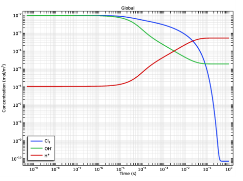
In the Settings window for Global, click Replace Expression in the upper-right corner of the y-Axis Data section. From the menu, choose Component 1 (comp1)>Reaction Engineering>re.c_Cl2 - Concentration - mol/m³.
3
Click Add Expression in the upper-right corner of the y-Axis Data section. From the menu, choose Component 1 (comp1)>Reaction Engineering>re.c_OH - Concentration - mol/m³.
4
Click Add Expression in the upper-right corner of the y-Axis Data section. From the menu, choose Component 1 (comp1)>Reaction Engineering>re.c_H - Concentration - mol/m³.
5
Click to expand the Coloring and Style section. In the Width text field, type 2.
6
Click to expand the Legends section. From the Legends list, choose Manual.
7
Concentration (re)
1
In the Model Builder window, click Concentration (re).
2
In the Settings window for 1D Plot Group, locate the Legend section.
3
From the Position list, choose Lower left.
4
In the Concentration (re) toolbar, click  Plot.
5
Click the  Zoom Extents button in the Graphics toolbar.