PDF

Carbon Deposition in Heterogeneous Catalysis
Introduction
Carbon deposition onto the surface of solid catalysts is commonly observed in hydrocarbon processing. Carbon deposits can affect both the activity of catalysts as well as the flow of gas through a catalyst bed.
This example investigates the thermal decomposition of methane into hydrogen and solid carbon with two models. In the first model, the isothermal process occurring in an ideal reactor is simulated with the Reaction Engineering interface. The influence of carbon deposition on catalyst activity is also considered. In the second model, the effect that the carbon deposits have on the porosity and the fluid flow is studied. The second simulation takes both time and space dependencies into account.
Model Definition
CHEMISTRY
Methane decomposes over a Ni/Al2O3 catalyst according to the overall chemical reaction
(1)
Under atmospheric pressure, the temperate ranging from 490 °C to 590 °C and a volume fraction of hydrogen between 0 and 40%, the following reaction rate expression has been reported in the literature (Ref. 1):
(2)
where
(3)
and
The constant k0 in Equation 3 is 2.31·105 mol/(m3·s), supposing the amount of catalyst being 1 g/m3. The unit for pressure in Equation 2 is bar.
IDEAL REACTOR MODEL
This model treats the isothermal decomposition of methane (Figure 2) in a perfectly mixed batch reactor with constant volume. The species mass balances are summarized by
The rate term, Ri (SI unit: mol/(m3·s)) for each species, takes into account the reaction stoichiometry coefficients, νi, the reaction rate reported in Equation 2, r mol/(m3·s), and the catalyst activity, a:
The mass balances of the reacting species are then
The time dependence of the catalytic activity is expressed by
where
where ka0 is 8.324·106 (m3/mol)3·s. Solving the mass balances provides the evolution of the species concentrations over time. The fact that carbon is in the solid phase is taken into account by removing its effect on gas phase physical properties. The pressure in the reactor is a function of only the methane and hydrogen concentrations:
SPACE- AND TIME-DEPENDENT MODEL
The second model takes fluid flow, mass transport, heat transfer, and the chemical reaction into account. It is created by the Generate Space-Dependent Model feature available in the Reaction Engineering interface.
:
Figure 1: Methane enters from the left and reacts in the porous catalytic bed in the porous catalytic bed of the geometry. The wall of the bed is heated.
Equations
The space-dependent model solves coupled momentum, mass, and energy balances together with a void fraction balance. The fluid flow is laminar, the concentrations high (no solvent is present), and porous media with variable porosity exist within the reactor. Additionally, the impact of heating is studied. The following physics interfaces are used in this example:
The Domain ODEs and PDEs interface solves a balance for the void fraction, or porosity, of the bed given by
where kpor is a constant, MC (kg/mol) is the carbon molar weight, and ρsoot (kg/m3) is the deposited carbon density. This equation can be implemented in the Domain ODEs and DAEs interface, resulting in a porosity distribution across the catalytic bed as a function of time. The initial porosity of the bed is assumed to be ε = 0.4.
The porosity is related to the permeability of the porous domain by (Ref. 2)
The reactor geometry (see Figure 1) is set up in 2D axisymmetry in the model as the angular gradients are negligible.
Results and Discussion
IDEAL REACTOR MODEL
Figure 2 shows the concentration transients of methane, hydrogen, and deposited carbon as methane decomposes over a Ni/Al2O3 catalyst. Both the composition with and without catalyst deactivation are displayed. From the change in concentrations with time, the reaction rate with constant catalyst activity is shown to be larger than when catalyst deactivation is accounted for.
Figure 2: Concentration transients of methane decomposition over a Ni/Al2O3 catalyst for two catalyst conditions: 1) deactivation; 2) constant activity.
Figure 3 shows the deactivation of catalyst during methane decomposition. The activity of catalyst decreases rapidly at the early stage of reaction, then decreases slowly.
Figure 3: Change of catalyst activity with reacting time.
SPACE- AND TIME-DEPENDENT MODEL
Figure 4 shows the velocity profile (surface) and pressure difference (contour) in the reactor at the end of the simulation. The flow velocity of gas is slower within the porous catalytic bed. The figure also displays a pressure drop across the bed.
Figure 4: Velocity flow field and pressure drop within the after 20,000 s. Surface plot displays the velocity (SI unit: m/s) and contour plot the pressure (SI unit: Pa).
Figure 5 shows the temperature distribution after 50 s and 500  s. It takes approximately 300 s for the bed to heat up to the same temperature as the walls (850 K).
Figure 5: Temperature distribution within the reactor after 50 s and 500 s.
Figure 6 shows a comparison of the concentration distributions for methane at 400 s and 4,000  s. The concentration of methane decreases more rapidly as soon as the bed is sufficiently heated (Figure 5).
Figure 6: Concentration distribution of methane within the reactor at 400 s and 4,000 s.
The concentration distribution of methane and hydrogen is displayed along the centerline of the porous catalyst bed in Figure 7. The figure shows in detail that the production of hydrogen varies with time and heating.
Figure 7: Concentration distribution of CH4 and H2 along the center of the porous catalyst bed at 50 s and 500 s.
Figure 8 illustrates that the porosity varies within the bed at 20,000 s and that the pores may become completely clogged near the bed inlet with time.
Figure 8: Porosity distribution within the porous catalyst bed at 4,000 s.
References
1. S.G. Zavarukhin and G.G. Kuvshinov, “The kinetic model of formation of nanofibrous carbon from CH4–H2 mixture over a high-loaded nickel catalyst with consideration for the catalyst deactivation”, J. Appl. Catal. A, vol. 272, pp. 219–227, 2004.
2. E.A. Borisova and P.M. Adler, “Deposition in porous media and clogging on the field scale”, Phys. Rev. E, vol. 71, p. 016311-1, 2005.
Application Library path: Chemical_Reaction_Engineering_Module/Reactors_with_Porous_Catalysts/carbon_deposition
Modeling Instructions
From the File menu, choose New.
New
In the New window, click  Model Wizard.
Model Wizard
1
In the Model Wizard window, click  0D.
2
In the Select Physics tree, select Chemical Species Transport>Reaction Engineering (re).
3
Click Add.
4
Click  Study.
5
In the Select Study tree, select General Studies>Time Dependent.
6
Reaction Engineering (re)
Reaction 1
1
In the Model Builder window, under Component 1 (comp1) right-click Reaction Engineering (re) and choose Reaction.
2
In the Settings window for Reaction, locate the Reaction Formula section.
3
In the Formula text field, type CH4=>C+2H2.
Species 1
Add an individual species representing the catalyst activity.
1
In the Reaction Engineering toolbar, click  Species.
2
In the Settings window for Species, locate the Species Name section.
3
When a new species is created a mass balance equation is set up along with it. Note that you can remove the effect of catalyst activity from your model by selecting the Lock concentration/activity check box.This removes the species mass balance and sets the concentration of the species to the value entered in the Initial Values node.
Global Definitions
Load the model parameters from a text file.
Parameters 1
1
In the Model Builder window, under Global Definitions click Parameters 1.
2
In the Settings window for Parameters, locate the Parameters section.
3
Click  Load from File.
4
Definitions
Load the model variables from a text file.
Variables 1
1
In the Model Builder window, under Component 1 (comp1) right-click Definitions and choose Variables.
2
In the Settings window for Variables, locate the Variables section.
3
Click  Load from File.
4
For the k variable definition above, it is assumed that there is 1 [g/m^3] catalyst.
Reaction Engineering (re)
1: CH4=>C+2H2
1
In the Model Builder window, under Component 1 (comp1)>Reaction Engineering (re) click 1: CH4=>C+2H2.
2
In the Settings window for Reaction, locate the Reaction Rate section.
3
4
In the rj text field, type re.c_a*k*(P_CH4-P_H2^2/Kp)/(1+kH*sqrt(P_H2))^2.
Additional Source 1
1
In the Reaction Engineering toolbar, click  Additional Source.
2
In the Settings window for Additional Source, locate the Additional Rate Expression section.
3
In the Volumetric species table, enter the following settings:
Initial Values 1
1
In the Model Builder window, click Initial Values 1.
2
In the Settings window for Initial Values, locate the Volumetric Species Initial Values section.
3
4
In the Model Builder window, click Reaction Engineering (re).
5
In the Settings window for Reaction Engineering, locate the Energy Balance section.
6
In the T text field, type 850[K].
7
Locate the Mixture Properties section. From the Reactor pressure list, choose User defined.
8
In the p text field, type R_const*re.T*(re.c_CH4+re.c_H2).
Study 1
Step 1: Time Dependent
1
In the Model Builder window, under Study 1 click Step 1: Time Dependent.
2
In the Settings window for Time Dependent, locate the Study Settings section.
3
In the Output times text field, type range(0,500,20000).
4
In the Home toolbar, click  Compute.
Study 1
Solution 1 (sol1)
1
In the Model Builder window, expand the Study 1>Solver Configurations node.
2
Right-click Solution 1 (sol1) and choose Solution>Copy.
With catalyst deactivation
1
In the Model Builder window, under Study 1>Solver Configurations click Solution 1 - Copy 1 (sol2).
2
In the Settings window for Solution, type With catalyst deactivation in the Label text field.
Results
Catalyst Activity (re)
1
In the Model Builder window, under Results click Concentration (re).
2
In the Settings window for 1D Plot Group, locate the Data section.
3
From the Dataset list, choose Study 1/With catalyst deactivation (sol2).
4
In the Label text field, type Catalyst Activity (re).
5
Click to expand the Title section. From the Title type list, choose Manual.
6
In the Title text area, type Catalyst activity.
Global 1
1
In the Model Builder window, expand the Catalyst Activity (re) node, then click Global 1.
2
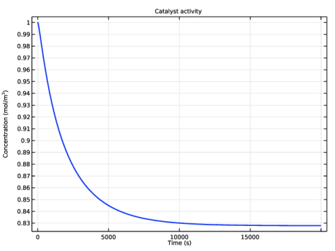
In the Settings window for Global, click Replace Expression in the upper-right corner of the y-Axis Data section. From the menu, choose Component 1 (comp1)>Reaction Engineering>re.c_a - Concentration - mol/m³.
3
Click to expand the Coloring and Style section. In the Width text field, type 2.
4
Click to expand the Legends section. Clear the Show legends check box.
5
In the Catalyst Activity (re) toolbar, click  Plot.
Now study the reaction when the catalyst activity is held constant (initial value).
Reaction Engineering (re)
Species: a
1
In the Model Builder window, under Component 1 (comp1)>Reaction Engineering (re) click Species: a.
2
In the Settings window for Species, click to expand the Species Concentration/Activity section.
3
Select the Constant concentration/activity check box.
Study 1
In the Home toolbar, click  Compute.
Solution 1 (sol1)
In the Model Builder window, under Study 1>Solver Configurations right-click Solution 1 (sol1) and choose Solution>Copy.
Constant catalyst activity
1
In the Model Builder window, under Study 1>Solver Configurations click Solution 1 - Copy 1 (sol3).
2
In the Settings window for Solution, type Constant catalyst activity in the Label text field.
Results
Compare the concentrations between locked (constant catalyst activity) and unlocked (with catalyst deactivation) species a.
Concentration Comparison (re)
1
In the Model Builder window, under Results click Concentration (re).
2
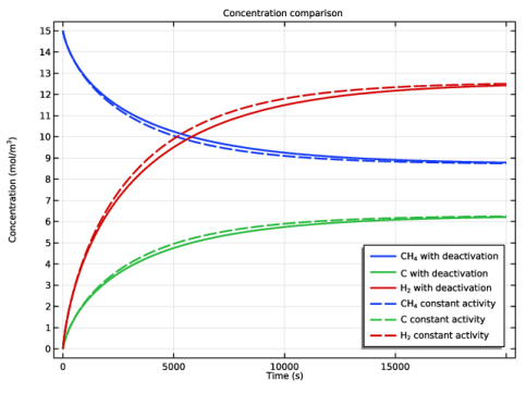
In the Settings window for 1D Plot Group, type Concentration Comparison (re) in the Label text field.
3
Locate the Title section. From the Title type list, choose Manual.
4
In the Title text area, type Concentration comparison.
5
Locate the Legend section. From the Position list, choose Lower right.
With catalyst deactivation
1
In the Model Builder window, expand the Concentration Comparison (re) node, then click Global 1.
2
In the Settings window for Global, type With catalyst deactivation in the Label text field.
3
Locate the Data section. From the Dataset list, choose Study 1/With catalyst deactivation (sol2).
4
Locate the Coloring and Style section. In the Width text field, type 2.
5
Locate the Legends section. From the Legends list, choose Manual.
6
Constant catalyst activity
1
Right-click With catalyst deactivation and choose Duplicate.
2
In the Settings window for Global, type Constant catalyst activity in the Label text field.
3
Locate the Data section. From the Dataset list, choose Study 1/Constant catalyst activity (sol3).
4
Locate the Coloring and Style section. Find the Line style subsection. From the Line list, choose Dashed.
5
From the Color list, choose Cycle (reset).
6
Locate the Legends section. In the table, enter the following settings:
7
In the Concentration Comparison (re) toolbar, click  Plot.
Create a time- and space-dependent model from the Reaction Engineering interface. All solid species should be locked before this is done.
Reaction Engineering (re)
Species: C
1
In the Model Builder window, under Component 1 (comp1)>Reaction Engineering (re) click Species: C.
2
In the Settings window for Species, locate the Species Concentration/Activity section.
3
Select the Constant concentration/activity check box.
Generate Space-Dependent Model 1
1
In the Reaction Engineering toolbar, click  Generate Space-Dependent Model.
2
In the Settings window for Generate Space-Dependent Model, locate the Component Settings section.
3
From the Component to use list, choose 2Daxi: New.
4
Locate the Physics Interfaces section. Find the Chemical species transport subsection. From the list, choose Transport of Concentrated Species: New.
5
Find the Heat transfer subsection. From the list, choose Heat Transfer in Porous Media: New.
6
Find the Fluid flow subsection. From the list, choose Laminar Flow: New.
7
Locate the Space-Dependent Model Generation section. Click Create/Refresh.
Definitions (comp2)
Add variables for the Chemistry node which are similar to those used in the Reaction Engineering interface.
Variables 2
1
In the Model Builder window, expand the Component 2 (comp2) node.
2
Right-click Component 2 (comp2)>Definitions and choose Variables.
3
In the Settings window for Variables, locate the Variables section.
4
Click  Load from File.
5
In order to get significant carbon deposition, the amount of catalyst is increased to 300 [g/m^3]. The k value is 300 times as that in 0D.
Geometry 1(2Daxi)
Rectangle 1 (r1)
1
In the Geometry toolbar, click  Rectangle.
2
In the Settings window for Rectangle, locate the Size and Shape section.
3
In the Width text field, type 0.01.
4
In the Height text field, type 0.04.
Rectangle 2 (r2)
1
In the Geometry toolbar, click  Rectangle.
2
In the Settings window for Rectangle, locate the Size and Shape section.
3
In the Width text field, type 0.015.
4
In the Height text field, type 0.12.
5
Locate the Position section. In the z text field, type 0.04.
Rectangle 3 (r3)
1
In the Geometry toolbar, click  Rectangle.
2
In the Settings window for Rectangle, locate the Size and Shape section.
3
In the Width text field, type 0.01.
4
In the Height text field, type 0.04.
5
Locate the Position section. In the z text field, type 0.16.
6
Click  Build All Objects.
Fillet 1 (fil1)
1
In the Geometry toolbar, click  Fillet.
2
On the object r2, select Points 2 and 3 only.
3
In the Settings window for Fillet, locate the Radius section.
4
In the Radius text field, type 0.001.
5
Click  Build All Objects.
Union 1 (uni1)
1
In the Geometry toolbar, click  Booleans and Partitions and choose Union.
2
Click in the Graphics window and then press Ctrl+A to select all objects.
3
In the Settings window for Union, locate the Union section.
4
Clear the Keep interior boundaries check box.
5
Click  Build All Objects.
Fillet 2 (fil2)
1
In the Geometry toolbar, click  Fillet.
2
On the object uni1, select Points 6 and 7 only.
3
In the Settings window for Fillet, locate the Radius section.
4
In the Radius text field, type 0.004.
Rectangle 4 (r4)
1
In the Geometry toolbar, click  Rectangle.
2
In the Settings window for Rectangle, locate the Size and Shape section.
3
In the Width text field, type 0.015.
4
In the Height text field, type 0.112.
5
Locate the Position section. In the z text field, type 0.044.
6
Click  Build All Objects.
7
Click the  Zoom Extents button in the Graphics toolbar.
Component 2 (comp2)
Add the Domain ODE and DAE interface for modeling of the porosity change in the porous domain.
Add Physics
1
In the Home toolbar, click  Add Physics to open the Add Physics window.
2
Go to the Add Physics window.
3
In the tree, select Mathematics>ODE and DAE Interfaces>Domain ODEs and DAEs (dode).
4
Click Add to Component 2 in the window toolbar.
5
In the Home toolbar, click  Add Physics to close the Add Physics window.
Porosity Change
1
In the Settings window for Domain ODEs and DAEs, type Porosity Change in the Label text field.
2
Locate the Domain Selection section. Click  Clear Selection.
3
4
Locate the Units section. In the Source term quantity table, enter the following settings:
5
Click to expand the Dependent Variables section. In the Field name text field, type por.
6
In the Dependent variables table, enter the following settings:
Distributed ODE 1
1
In the Model Builder window, under Component 2 (comp2)>Porosity Change (dode) click Distributed ODE 1.
2
In the Settings window for Distributed ODE, locate the Source Term section.
3
In the f text field, type -por*chem.r_1*chem.M_C/rho_soot.
Initial Values 1
1
In the Model Builder window, click Initial Values 1.
2
In the Settings window for Initial Values, locate the Initial Values section.
3
In the por text field, type por0.
Chemistry 1 (chem)
Species: CH4
1
In the Model Builder window, expand the Component 2 (comp2)>Chemistry 1 (chem) node, then click Species: CH4.
2
In the Settings window for Species, click to expand the Species Transport Expressions section.
3
From the Thermal conductivity list, choose User defined.
4
In the k text field, type kt_CH4.
5
Click to expand the Species Thermodynamic Expressions section. From the list, choose User defined.
6
In the Cp text field, type Cp_CH4*chem.M_CH4.
7
In the h text field, type h_CH4.
8
In the s text field, type s_CH4.
Species: H2
1
In the Model Builder window, click Species: H2.
2
In the Settings window for Species, locate the Species Transport Expressions section.
3
From the Thermal conductivity list, choose User defined.
4
In the k text field, type kt_H2.
5
Locate the Species Thermodynamic Expressions section. From the list, choose User defined.
6
In the Cp text field, type Cp_H2*chem.M_H2.
7
In the h text field, type h_H2.
8
In the s text field, type s_H2.
Species: C
1
In the Model Builder window, click Species: C.
2
In the Settings window for Species, locate the Species Transport Expressions section.
3
From the Thermal conductivity list, choose User defined.
4
In the k text field, type kt_C.
5
Locate the Species Thermodynamic Expressions section. From the list, choose User defined.
6
In the Cp text field, type Cp_C*chem.M_C.
7
In the h text field, type h_C.
8
In the s text field, type s_C.
Species: a
1
In the Model Builder window, click Species: a.
2
In the Settings window for Species, locate the General Parameters section.
3
In the M text field, type M_a.
4
Locate the Species Transport Expressions section. From the Thermal conductivity list, choose User defined.
5
In the k text field, type kt_cat.
Transport of Concentrated Species (tcs)
1
In the Model Builder window, under Component 2 (comp2) click Transport of Concentrated Species (tcs).
2
In the Settings window for Transport of Concentrated Species, locate the Transport Mechanisms section.
3
Select the Mass transfer in porous media check box.
Transport Properties 1
1
In the Model Builder window, expand the Transport of Concentrated Species (tcs) node, then click Transport Properties 1.
2
In the Settings window for Transport Properties, locate the Diffusion section.
3
Reaction Sources 1
1
In the Model Builder window, click Reaction Sources 1.
2
3
In the Settings window for Reaction Sources, locate the Domain Selection section.
4
Click  Remove from Selection.
5
6
Locate the Reacting Volume section. From the Reacting volume list, choose Pore volume.
Inflow 1
1
In the Physics toolbar, click  Boundaries and choose Inflow.
2
3
In the Settings window for Inflow, locate the Inflow section.
4
In the ω0,wH2 text field, type 0.
Outflow 1
1
In the Physics toolbar, click  Boundaries and choose Outflow.
2
Porous Medium 1
1
In the Physics toolbar, click  Domains and choose Porous Medium.
2
Fluid 1
1
In the Model Builder window, click Fluid 1.
2
In the Settings window for Fluid, click to expand the Model Input section.
3
From the pA list, choose Absolute pressure (spf).
4
Locate the Convection section. From the u list, choose Velocity field (spf).
5
Locate the Density section. From the MwCH4 list, choose Molar mass (chem/CH4).
6
From the MwH2 list, choose Molar mass (chem/H2).
7
Locate the Diffusion section. In the table, enter the following settings:
Porous Matrix 1
1
In the Model Builder window, click Porous Matrix 1.
2
In the Settings window for Porous Matrix, locate the Matrix Properties section.
3
In the εp text field, type por.
Heat Transfer in Porous Media 1 (ht)
Fluid 1
1
In the Model Builder window, expand the Component 2 (comp2)>Heat Transfer in Porous Media 1 (ht)>Porous Medium 1 node, then click Fluid 1.
2
In the Settings window for Fluid, locate the Thermodynamics, Fluid section.
3
From the Mn list, choose Mean molar mass (chem).
Porous Matrix 1
1
In the Model Builder window, click Porous Matrix 1.
2
In the Settings window for Porous Matrix, locate the Matrix Properties section.
3
From the εp list, choose User defined. In the associated text field, type por.
4
From the Define list, choose Solid phase properties.
5
Locate the Heat Conduction, Porous Matrix section. From the ks list, choose User defined. In the associated text field, type kt_cat.
6
Locate the Thermodynamics, Porous Matrix section. From the ρs list, choose User defined. In the associated text field, type rho_cat.
7
From the Cp,s list, choose User defined. In the associated text field, type Cp_cat.
Heat Source 1
1
In the Model Builder window, under Component 2 (comp2)>Heat Transfer in Porous Media 1 (ht) click Heat Source 1.
2
3
In the Settings window for Heat Source, locate the Heat Source section.
4
In the Q0 text field, type chem.Qtot*por.
Temperature 1
1
In the Physics toolbar, click  Boundaries and choose Temperature.
2
Outflow 1
1
In the Physics toolbar, click  Boundaries and choose Outflow.
2
Temperature 2
1
In the Physics toolbar, click  Boundaries and choose Temperature.
2
3
In the Settings window for Temperature, locate the Temperature section.
4
In the T0 text field, type 850[K].
Fluid 1
1
In the Physics toolbar, click  Domains and choose Fluid.
2
3
In the Settings window for Fluid, locate the Heat Convection section.
4
From the u list, choose Velocity field (spf).
5
Locate the Heat Conduction, Fluid section. From the k list, choose Thermal conductivity (chem).
6
Locate the Thermodynamics, Fluid section. From the Fluid type list, choose Gas/Liquid.
7
From the ρ list, choose Density (chem).
8
From the Cp list, choose Heat capacity at constant pressure (chem).
9
From the γ list, choose User defined.
Laminar Flow 1 (spf)
1
In the Model Builder window, under Component 2 (comp2) click Laminar Flow 1 (spf).
2
In the Settings window for Laminar Flow, locate the Physical Model section.
3
Select the Enable porous media domains check box.
Fluid Properties 1
1
In the Model Builder window, expand the Laminar Flow 1 (spf) node, then click Fluid Properties 1.
2
In the Settings window for Fluid Properties, locate the Fluid Properties section.
3
From the ρ list, choose Density (chem).
Porous Medium 1
1
In the Physics toolbar, click  Domains and choose Porous Medium.
2
Fluid 1
1
In the Model Builder window, expand the Porous Medium 1 node, then click Fluid 1.
2
In the Settings window for Fluid, locate the Fluid Properties section.
3
From the ρ list, choose Density (chem).
4
From the μ list, choose Dynamic viscosity (chem).
Porous Matrix 1
1
In the Model Builder window, click Porous Matrix 1.
2
In the Settings window for Porous Matrix, locate the Matrix Properties section.
3
From the εp list, choose User defined. In the associated text field, type por.
4
From the κ list, choose User defined. In the associated text field, type kappa.
Inlet 1
1
In the Physics toolbar, click  Boundaries and choose Inlet.
2
3
In the Settings window for Inlet, locate the Boundary Condition section.
4
From the list, choose Fully developed flow.
5
Locate the Fully Developed Flow section. In the Uav text field, type u_in.
Outlet 1
1
In the Physics toolbar, click  Boundaries and choose Outlet.
2
Mass Source 1
1
In the Physics toolbar, click  Domains and choose Mass Source.
2
3
In the Settings window for Mass Source, locate the Mass Source section.
4
In the Qm text field, type (chem.Rw_CH4+chem.Rw_H2)*por.
Study 2
Step 1: Stationary
1
In the Model Builder window, expand the Study 2 node, then click Step 1: Stationary.
2
In the Settings window for Stationary, locate the Physics and Variables Selection section.
3
In the table, clear the Solve for check boxes for Chemistry 1 (chem), Transport of Concentrated Species (tcs), Heat Transfer in Porous Media 1 (ht), and Porosity Change (dode).
Time Dependent
1
In the Study toolbar, click  Study Steps and choose Time Dependent>Time Dependent.
2
In the Settings window for Time Dependent, locate the Study Settings section.
3
In the Output times text field, type range(0,50,1000) range(2000,1000,20000).
4
Locate the Physics and Variables Selection section. In the table, clear the Solve for check box for Reaction Engineering (re).
5
In the Study toolbar, click  Compute.
Results
Temperature, 3D
1
In the Model Builder window, under Results click Temperature, 3D (ht1).
2
In the Settings window for 3D Plot Group, type Temperature, 3D in the Label text field.
3
Locate the Data section. From the Time (s) list, choose 50.
4
Locate the Plot Settings section. Clear the Plot dataset edges check box.
Surface
1
In the Model Builder window, expand the Temperature, 3D node, then click Surface.
2
In the Settings window for Surface, locate the Coloring and Style section.
3
From the Color table list, choose ThermalDark.
4
Click Replace Expression in the upper-right corner of the Expression section. From the menu, choose Component 2 (comp2)>Heat Transfer in Porous Media 1>Temperature>T - Temperature - K.
Adjust the view angle of the plot with the mouse.
Temperature, 3D
1
In the Model Builder window, click Temperature, 3D.
2
In the Temperature, 3D toolbar, click  Plot.
3
Click the  Zoom Extents button in the Graphics toolbar.
4
In the Settings window for 3D Plot Group, locate the Data section.
5
From the Time (s) list, choose 500.
6
In the Temperature, 3D toolbar, click  Plot.
7
Click the  Zoom Extents button in the Graphics toolbar.
Concentration, CH4, 3D (tcs)
1
In the Model Builder window, click Concentration, CH4, 3D (tcs).
2
In the Settings window for 3D Plot Group, locate the Data section.
3
From the Time (s) list, choose 50.
4
Click to expand the Title section. Locate the Plot Settings section. Clear the Plot dataset edges check box.
5
In the Concentration, CH4, 3D (tcs) toolbar, click  Plot.
6
Click the  Zoom Extents button in the Graphics toolbar.
7
Locate the Data section. From the Time (s) list, choose 500.
8
In the Concentration, CH4, 3D (tcs) toolbar, click  Plot.
9
Click the  Zoom Extents button in the Graphics toolbar.
Velocity, 3D (spf1)
1
In the Model Builder window, click Velocity, 3D (spf1).
2
In the Settings window for 3D Plot Group, locate the Plot Settings section.
3
Clear the Plot dataset edges check box.
Contour 1
1
Right-click Velocity, 3D (spf1) and choose Contour.
2
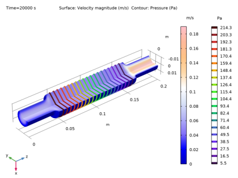
In the Settings window for Contour, click Replace Expression in the upper-right corner of the Expression section. From the menu, choose Component 2 (comp2)>Laminar Flow 1>Velocity and pressure>p - Pressure - Pa.
3
Click to expand the Title section. Locate the Coloring and Style section. From the Contour type list, choose Tube.
4
From the Color table list, choose Spectrum.
Surface
1
In the Model Builder window, click Surface.
2
In the Settings window for Surface, locate the Coloring and Style section.
3
From the Color table list, choose Twilight.
4
From the Color table transformation list, choose Reverse.
Velocity, 3D (spf1)
1
In the Model Builder window, click Velocity, 3D (spf1).
2
In the Settings window for 3D Plot Group, locate the Color Legend section.
3
Select the Show units check box.
4
In the Velocity, 3D (spf1) toolbar, click  Plot.
5
Click the  Zoom Extents button in the Graphics toolbar.
Cut Line 3D 1
1
In the Results toolbar, click  Cut Line 3D.
2
In the Settings window for Cut Line 3D, locate the Line Data section.
3
In row Point 1, set z to 0.044.
4
In row Point 2, set x to 0 and z to 0.156.
Concentration CH4, Porous Catalyst Bed Center
1
In the Results toolbar, click  1D Plot Group.
2
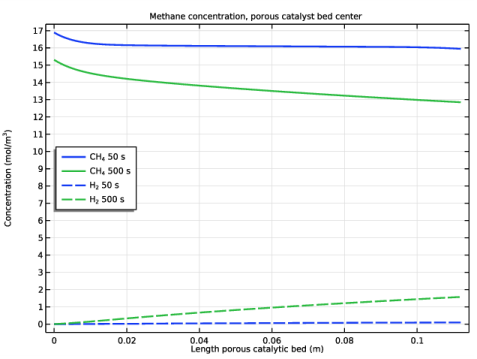
In the Settings window for 1D Plot Group, type Concentration CH4, Porous Catalyst Bed Center in the Label text field.
3
Locate the Data section. From the Dataset list, choose Cut Line 3D 1.
4
From the Time selection list, choose From list.
5
In the Times (s) list, choose 50 and 500.
6
Locate the Title section. From the Title type list, choose Manual.
7
In the Title text area, type Methane concentration, porous catalyst bed center.
8
Locate the Plot Settings section. Select the x-axis label check box.
9
In the associated text field, type Length porous catalytic bed (m).
10
Select the y-axis label check box.
11
In the associated text field, type Concentration (mol/m<sup>3</sup>).
12
Locate the Legend section. From the Position list, choose Middle left.
Line Graph 1
1
Right-click Concentration CH4, Porous Catalyst Bed Center and choose Line Graph.
2
In the Settings window for Line Graph, click Replace Expression in the upper-right corner of the y-Axis Data section. From the menu, choose Component 2 (comp2)>Transport of Concentrated Species>Species wCH4>tcs.c_wCH4 - Molar concentration - mol/m³.
3
Click to expand the Coloring and Style section. In the Width text field, type 2.
4
Click to expand the Legends section. Select the Show legends check box.
5
From the Legends list, choose Evaluated.
6
In the Legend text field, type CH<sub>4</sub> eval(t,s) s.
Line Graph 2
1
Right-click Line Graph 1 and choose Duplicate.
2
In the Settings window for Line Graph, click Replace Expression in the upper-right corner of the y-Axis Data section. From the menu, choose Component 2 (comp2)>Transport of Concentrated Species>Species wH2>tcs.c_wH2 - Molar concentration - mol/m³.
3
Locate the Coloring and Style section. Find the Line style subsection. From the Line list, choose Dashed.
4
From the Color list, choose Cycle (reset).
5
Locate the Legends section. In the Legend text field, type H<sub>2</sub> eval(t,s) s.
6
In the Concentration CH4, Porous Catalyst Bed Center toolbar, click  Plot.
Porosity Distribution
1
In the Model Builder window, under Results click 3D Plot Group 13.
2
In the Settings window for 3D Plot Group, type Porosity Distribution in the Label text field.
3
Locate the Title section. From the Title type list, choose Manual.
4
In the Title text area, type Porosity within porous catalyst bed.
5
In the Porosity Distribution toolbar, click  Plot.
6
Click the  Zoom Extents button in the Graphics toolbar.
Delete the .
For future use of Study 1, turn off the interfaces associated with the space-dependent model.
Study 1
Step 1: Time Dependent
1
In the Model Builder window, under Study 1 click Step 1: Time Dependent.
2
In the Settings window for Time Dependent, locate the Physics and Variables Selection section.
3
In the table, clear the Solve for check boxes for Chemistry 1 (chem), Transport of Concentrated Species (tcs), Heat Transfer in Porous Media 1 (ht), Laminar Flow 1 (spf), and Porosity Change (dode).
The 2D plot group showing the porosity is not needed and can be deleted.
Results
2D Plot Group 12
In the Model Builder window, under Results right-click 2D Plot Group 12 and choose Delete.