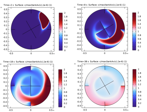
PDF

Turbulent Mixing in a Stirred Tank
Introduction
This tutorial demonstrates how mixing can be simulated in a stirred vessel by seeding a trace species from a point. The flow is modeled using the Rotating Machinery, Fluid Flow interface, which solves the Navier-Stokes equations on geometries with rotating parts such as impellers. The transport of the trace species is modeled using the Transport of Diluted Species interface. The trace species is added when the mixer is running in steady operation. The mixing time is evaluated by comparing the concentration in a measurement point to the average concentration in the vessel.
Model Definition
Model Geometry
Figure 1 shows the model geometry, which is a schematic cross section of a tank with a four-blade impeller. The tank has four baffles attached to the wall to enhance mixing. The mixer blades and the impellers are approximated to be infinitely thin. The seeding of the trace species is done at the marked seeding point. The tank also contains a measurement point, close to the wall, where the concentration can be probed.
The circle between the impeller and the tank wall is the assembly boundary where the mesh is allowed to slide when the impeller rotates.
Figure 1: Model geometry.
Domain Equation and Boundary Conditions
The mixer fluid is water, and a rotational speed of 20 rpm is prescribed for the impeller. This rotation is achieved by prescribing the inner domain to be a rotating domain. The boundary between the inner and the outer domain is prescribed to be a continuity boundary that transfers momentum to the fluid in the outer domain.
The Reynolds number based on the impeller radius and the impeller tip speed is approximately 1.9 × 106, which means that the flow is turbulent. The kε turbulence model is applied in this example.
There are two methods to reach operating conditions. One is to accelerate the impeller up to full speed and wait for the flow to reach a quasi steady-state. This approach is simple but can be time consuming. A computationally more efficient method is to first simulate the flow using the frozen rotor approach. Frozen rotor means that the impeller, or rotor, is frozen in position. The flow in the rotating domain is assumed to be stationary in terms of a rotating coordinate system. The effect of the rotation is then accounted for by Coriolis and centrifugal forces. This solution couples to the nonrotating parts where the flow is also assumed to be stationary, but in a nonrotating coordinate system. See the CFD Module User’s Guide for more information about frozen rotor.
The result of a frozen rotor simulation is an approximation to the flow at operating conditions. The result depends on the angular position of the impeller and cannot represent transient effects. It is still a very good starting condition to reach operating conditions. Here, to make sure that the correct operating conditions are reached, a time dependent simulations in ran starting from the frozen rotor solution. The average flow quantities are inspected in order to determine when a quasi-steady state is reached.
A trace species is a species introduced in very small quantities. It is often of a sharp color to be clearly visible even in small amounts. A trace species is not supposed to affect the flow, and hence, the flow can be solved for first and then the trace species transport solved for subsequently. The seeding is performed by injection at the seeding point during one second. Then the mixing in the vessel is simulated for 40 revolutions. The degree of mixing is evaluated by comparing the averaged concentration to the concentration measured near the wall behind one of the baffles.
To reduce the computational effort, the fluid flow field is not solved for during the mixing. The flow field and turbulent diffusion during the last revolution of the flow simulation is reused repeatedly during the mixing stage.
Note that in order to be able to reuse the flow field in a periodic fashion, variables are re-defined in the Equation View of the multiphysics coupling feature (Reacting Flow, Diluted Species).
Results and Discussion
Figure 2 shows the frozen rotor velocity field. As expected, the highest velocity magnitude is found at the tip of the mixer blades. There are also clearly visible recirculation zones both before and behind the baffles.
Figure 3 shows the velocity field at the end of the fluid flow simulation (at = 30 s, corresponding to 10 revolutions). The rotor position is the same as in Figure 2, and the results in the figures are similar. There are, however, differences. The most notably difference is the recirculation zones before the baffles that are smaller in Figure 3 than in Figure 2. The size and shape of the recirculation zones for the time-dependent simulation also vary with the position of the impeller.
Figure 2: The velocity field obtained from the frozen rotor simulation.
Figure 3: A snapshot of the time-dependent velocity field at t=30 s.
The average velocity and the average turbulent dynamic viscosity are plotted in Figure 4 to visualize the flow field development over time. The variables are normalized using the results from the frozen rotor solution. It can be noted that there is a drift over the first couple of rotations, but the magnitude of the variations are small. The frequency with which the impeller blades are passing the baffles is clearly seen in the velocity variations. The flow is noted to reached a cyclic steady state after around seven revolutions. This implies that the last revolution of the simulation can confidently be used repeatedly for the mixing simulation.
Figure 4: Flow development starting from the frozen rotor solution. The average velocity and average turbulent diffusion normalized by the respective initial value are shown.
Figure 5 shows four snapshots of the mixing process, with the time running from the upper-left to the lower-right picture. Since the velocity is rather slow at the seeding point (see also Figure 3), the initial transport is almost isotropic around the seeding point (t = 2 s). Some trace species is, however, entrained in the faster velocity field in the center of the mixer and becomes thereby spread in the azimuthal direction (t = 8 s). The slowest spreading is to the regions behind the left baffle, close to the measuring point, as well as behind the top baffle. The mixing in also poor in between the impeller blades. This is a well-known phenomenon and is the reason to why chemical substances are commonly added as close to the impeller axis as possible.
Figure 5: The mixing process. Surface plots of the trace species, normalized by the average concentration, at t = 2, 8, 18 and 38 seconds.
The mixing development can be evaluated in Figure 5 where the concentration at the measurement position and the average concentration are plotted. As was noted in the previous figure it takes a number of rotations of the impeller before the species is spread to the measurement position. After about 14 rotations the concentration behind the baffle surpasses the averaged concentrations, and after around 30 rotations the average concentration has been reached.
Figure 6: Concentration development during mixing. Comparing the average concentration in the tank to the one in the measurement point.
Application Library path: CFD_Module/Single-Phase_Flow/turbulent_mixing
Modeling Instructions
From the File menu, choose New.
New
In the New window, click  Model Wizard.
Model Wizard
1
In the Model Wizard window, click  2D.
2
In the Select Physics tree, select Fluid Flow>Single-Phase Flow>Rotating Machinery, Fluid Flow>Turbulent Flow>Turbulent Flow, k-ε.
3
Click Add.
4
Click  Study.
5
In the Select Study tree, select Preset Studies for Selected Physics Interfaces>Frozen Rotor.
6
Global Definitions
Import some model parameters from a text file.
Parameters 1
1
In the Model Builder window, under Global Definitions click Parameters 1.
2
In the Settings window for Parameters, locate the Parameters section.
3
Click  Load from File.
4
Geometry 1
Circle 1 (c1)
1
In the Geometry toolbar, click  Circle.
2
In the Settings window for Circle, locate the Size and Shape section.
3
In the Radius text field, type tank_R.
Circle 2 (c2)
1
In the Geometry toolbar, click  Circle.
2
In the Settings window for Circle, locate the Size and Shape section.
3
In the Radius text field, type 0.7*tank_R.
4
Click  Build Selected.
Difference 1 (dif1)
1
In the Geometry toolbar, click  Booleans and Partitions and choose Difference.
2
In the Settings window for Difference, locate the Difference section.
3
Select the Keep objects to subtract check box.
4
5
Find the Objects to subtract subsection. Click to select the  Activate Selection toggle button.
6
Line Segment 1 (ls1)
1
In the Geometry toolbar, click  More Primitives and choose Line Segment.
2
In the Settings window for Line Segment, locate the Starting Point section.
3
From the Specify list, choose Coordinates.
4
Locate the Endpoint section. From the Specify list, choose Coordinates.
5
Locate the Starting Point section. In the x text field, type -tank_R.
6
Locate the Endpoint section. In the x text field, type -tank_R+baffle_L.
Rotate 1 (rot1)
1
In the Geometry toolbar, click  Transforms and choose Rotate.
2
3
In the Settings window for Rotate, locate the Rotation section.
4
Click  Range.
5
In the Range dialog box, type 90 in the Start text field.
6
In the Step text field, type 90.
7
In the Stop text field, type 270.
8
Click Replace.
9
In the Settings window for Rotate, locate the Input section.
10
Select the Keep input objects check box.
Point 1 (pt1)
1
In the Geometry toolbar, click  Point.
2
In the Settings window for Point, locate the Point section.
3
In the x text field, type inject_x.
4
In the y text field, type inject_y.
5
Click  Build Selected.
Point 2 (pt2)
1
In the Geometry toolbar, click  Point.
2
In the Settings window for Point, locate the Point section.
3
In the x text field, type -tank_R*0.97.
4
In the y text field, type 0.
5
Click  Build Selected.
Rotate 2 (rot2)
1
In the Geometry toolbar, click  Transforms and choose Rotate.
2
3
In the Settings window for Rotate, locate the Rotation section.
4
In the Angle text field, type -10.
5
Click  Build Selected.
Union 1 (uni1)
1
In the Geometry toolbar, click  Booleans and Partitions and choose Union.
The final operation will later be set to Form an assembly. Union operations are therefore necessary to merge the domains and the lines.
2
Select the objects dif1, ls1, pt1, rot1(1), rot1(2), rot1(3), and rot2 only.
Line Segment 2 (ls2)
1
In the Geometry toolbar, click  More Primitives and choose Line Segment.
2
In the Settings window for Line Segment, locate the Starting Point section.
3
From the Specify list, choose Coordinates.
4
Locate the Endpoint section. From the Specify list, choose Coordinates.
5
Locate the Starting Point section. In the x text field, type -0.25.
6
Locate the Endpoint section. In the x text field, type 0.25.
Line Segment 3 (ls3)
1
In the Geometry toolbar, click  More Primitives and choose Line Segment.
2
In the Settings window for Line Segment, locate the Starting Point section.
3
From the Specify list, choose Coordinates.
4
Locate the Endpoint section. From the Specify list, choose Coordinates.
5
Locate the Starting Point section. In the y text field, type -0.25.
6
Locate the Endpoint section. In the y text field, type 0.25.
Union 2 (uni2)
1
In the Geometry toolbar, click  Booleans and Partitions and choose Union.
2
Select the objects c2, ls2, and ls3 only.
Form Union (fin)
The boundary between the rotating and nonrotating domain must be an assembly boundary so that the parts can move relative to each other.
1
In the Model Builder window, under Component 1 (comp1)>Geometry 1 click Form Union (fin).
2
In the Settings window for Form Union/Assembly, locate the Form Union/Assembly section.
3
From the Action list, choose Form an assembly.
4
In the Geometry toolbar, click  Build All.
5
Click the  Zoom Extents button in the Graphics toolbar.
Create a selection for the interior boundaries representing the impeller and baffles.
Definitions
Impeller and Baffles
1
In the Definitions toolbar, click  Explicit.
2
In the Settings window for Explicit, locate the Input Entities section.
3
From the Geometric entity level list, choose Boundary.
4
5
In the Label text field, type Impeller and Baffles.
Create an average operator to be used for computing average quantities in the tank.
Average 1 (aveop1)
1
In the Definitions toolbar, click  Nonlocal Couplings and choose Average.
2
In the Settings window for Average, type tankAv in the Operator name text field.
3
Locate the Source Selection section. From the Selection list, choose All domains.
Add Material
1
In the Home toolbar, click  Add Material to open the Add Material window.
2
Go to the Add Material window.
3
In the tree, select Built-in>Water, liquid.
4
Click Add to Component in the window toolbar.
5
In the Home toolbar, click  Add Material to close the Add Material window.
Moving Mesh
Rotating Domain 1
1
In the Model Builder window, under Component 1 (comp1)>Moving Mesh click Rotating Domain 1.
2
3
In the Settings window for Rotating Domain, locate the Rotation section.
4
In the f text field, type -rpm.
Turbulent Flow, k-ε (spf)
Interior Wall 1
1
In the Model Builder window, under Component 1 (comp1) right-click Turbulent Flow, k-ε (spf) and choose Interior Wall.
2
In the Settings window for Interior Wall, locate the Boundary Selection section.
3
From the Selection list, choose Impeller and Baffles.
Pressure Point Constraint 1
1
In the Physics toolbar, click  Points and choose Pressure Point Constraint.
2
The pressure level must be specified to obtain a unique solution since water is an incompressible liquid.
Hide the internal boundaries between the moving and the stationary part of the geometry. First copy the boundary selection from the continuity feature.
Flow Continuity 1
1
In the Model Builder window, click Flow Continuity 1.
2
In the Settings window for Flow Continuity, click to expand the Boundary Selection section.
3
Click  Copy Selection.
Definitions
Hide for Physics 1
1
In the Model Builder window, right-click View 1 and choose Hide for Physics.
2
In the Settings window for Hide for Physics, locate the Geometric Entity Selection section.
3
From the Geometric entity level list, choose Boundary.
4
Click  Paste Selection.
5
In the Paste Selection dialog box, Press CTRL+V to paste the copied boundary selection.
6
Mesh 1
1
In the Model Builder window, under Component 1 (comp1) click Mesh 1.
2
In the Settings window for Mesh, locate the Physics-Controlled Mesh section.
3
From the Element size list, choose Fine.
Size
Right-click Component 1 (comp1)>Mesh 1 and choose Edit Physics-Induced Sequence.
Size 1
1
In the Model Builder window, right-click Free Triangular 1 and choose Size.
2
In the Settings window for Size, locate the Geometric Entity Selection section.
3
From the Geometric entity level list, choose Point.
4
5
Locate the Element Size section. Click the Custom button.
6
Locate the Element Size Parameters section. Select the Maximum element size check box.
7
8
Click  Build All.
Study 1
Step 1: Frozen Rotor
In the Home toolbar, click  Compute.
Results
Velocity (spf)
Create Figure 2 using the following steps.
Streamline 1
1
Right-click Velocity (spf) and choose Streamline.
2
In the Settings window for Streamline, locate the Streamline Positioning section.
3
From the Positioning list, choose Uniform density.
4
In the Separating distance text field, type 0.02.
5
Locate the Coloring and Style section. Find the Point style subsection. From the Color list, choose White.
6
In the Velocity (spf) toolbar, click  Plot.
Add a Time Dependent study.
Pressure (spf), Velocity (spf), Wall Resolution (spf)
1
In the Model Builder window, under Results, Ctrl-click to select Velocity (spf), Pressure (spf), and Wall Resolution (spf).
2
Fluid Flow, Frozen Rotor
In the Settings window for Group, type Fluid Flow, Frozen Rotor in the Label text field.
Add Study
1
In the Home toolbar, click  Add Study to open the Add Study window.
2
Go to the Add Study window.
3
Find the Studies subsection. In the Select Study tree, select General Studies>Time Dependent.
4
Click Add Study in the window toolbar.
5
In the Home toolbar, click  Add Study to close the Add Study window.
Definitions
Variables 1
1
In the Model Builder window, right-click Definitions and choose Variables.
2
In the Settings window for Variables, locate the Variables section.
3
Domain Probe: U
1
In the Definitions toolbar, click  Probes and choose Domain Probe.
2
In the Settings window for Domain Probe, type Domain Probe: U in the Label text field.
3
Locate the Expression section. In the Expression text field, type spf.U/U0.
Domain Probe: muT
1
Right-click Domain Probe: U and choose Duplicate.
2
In the Settings window for Domain Probe, type Domain Probe: muT in the Label text field.
3
Locate the Expression section. In the Expression text field, type spf.muT/muT0.
Study 2
In the Study toolbar, click  Show Default Plots.
Step 1: Time Dependent
Store time steps at the end of the simulation when the flow field is expected to have reached a quasi-steady state.
1
In the Model Builder window, under Study 2 click Step 1: Time Dependent.
2
In the Settings window for Time Dependent, locate the Study Settings section.
3
In the Output times text field, type 0 range(frev_t0,rev_dt,frev_tEnd).
Enable results while solving, and use the probes to monitor when a quasi-steady state is reached.
4
Click to expand the Results While Solving section. Select the Plot check box.
5
From the Plot group list, choose Velocity (spf) 1.
6
From the Update at list, choose Time steps taken by solver.
7
From the Probes list, choose Manual.
Start from the frozen rotor solution.
8
Click to expand the Values of Dependent Variables section. Find the Initial values of variables solved for subsection. From the Settings list, choose User controlled.
9
From the Method list, choose Solution.
10
From the Study list, choose Study 1, Frozen Rotor.
11
In the Study toolbar, click  Compute.
Results
Pressure (spf) 1, Probe Plot Group 7, Velocity (spf) 1, Wall Resolution (spf) 1
1
In the Model Builder window, under Results, Ctrl-click to select Velocity (spf) 1, Pressure (spf) 1, Wall Resolution (spf) 1, and Probe Plot Group 7.
2
Fluid Flow, Time Dependent
In the Settings window for Group, type Fluid Flow, Time Dependent in the Label text field.
Probe Plot Group 7
1
In the Model Builder window, click Probe Plot Group 7.
2
In the Settings window for 1D Plot Group, locate the Legend section.
3
From the Position list, choose Lower right.
Probe Table Graph 1
1
In the Model Builder window, expand the Probe Plot Group 7 node, then click Probe Table Graph 1.
2
In the Settings window for Table Graph, click to expand the Preprocessing section.
3
Find the x-axis column subsection. From the Preprocessing list, choose Linear.
4
In the Scaling text field, type rpm.
Probe Plot: Fluid flow development
1
In the Model Builder window, under Results>Fluid Flow, Time Dependent click Probe Plot Group 7.
2
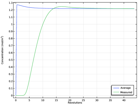
In the Settings window for 1D Plot Group, type Probe Plot: Fluid flow development in the Label text field.
3
Locate the Plot Settings section. Select the x-axis label check box.
4
Probe Table Graph 1
1
In the Model Builder window, expand the Probe Plot: Fluid flow development node, then click Probe Table Graph 1.
2
In the Settings window for Table Graph, click to expand the Legends section.
3
From the Legends list, choose Manual.
4
5
In the Probe Plot: Fluid flow development toolbar, click  Plot.
Velocity (spf) 1
Recreate Figure 3 using the following steps.
Streamline 1
1
In the Model Builder window, right-click Velocity (spf) 1 and choose Streamline.
2
In the Settings window for Streamline, locate the Streamline Positioning section.
3
From the Positioning list, choose Uniform density.
4
In the Separating distance text field, type 0.02.
5
Locate the Coloring and Style section. Find the Point style subsection. From the Color list, choose White.
6
In the Velocity (spf) 1 toolbar, click  Plot.
Definitions
Rectangle 1 (rect1)
1
In the Home toolbar, click  Functions and choose Local>Rectangle.
2
In the Settings window for Rectangle, locate the Parameters section.
3
In the Lower limit text field, type 0.1.
4
In the Upper limit text field, type 1.1.
5
Click to expand the Smoothing section. In the Size of transition zone text field, type 0.2.
Add Physics
1
In the Home toolbar, click  Add Physics to open the Add Physics window.
2
Go to the Add Physics window.
3
In the tree, select Chemical Species Transport>Transport of Diluted Species (tds).
4
Find the Physics interfaces in study subsection. In the table, clear the Solve check boxes for Study 1 and Study 2.
5
Click Add to Component 1 in the window toolbar.
6
In the Home toolbar, click  Add Physics to close the Add Physics window.
Multiphysics
Reacting Flow, Diluted Species 1 (rfd1)
In the Physics toolbar, click  Multiphysics Couplings and choose Domain>Reacting Flow, Diluted Species.
Add Study
1
In the Home toolbar, click  Add Study to open the Add Study window.
2
Go to the Add Study window.
3
Find the Studies subsection. In the Select Study tree, select General Studies>Time Dependent.
4
Find the Physics interfaces in study subsection. In the table, clear the Solve check box for Turbulent Flow, k-ε (spf).
5
Click Add Study in the window toolbar.
6
In the Home toolbar, click  Add Study to close the Add Study window.
Transport of Diluted Species (tds)
In the Model Builder window, under Component 1 (comp1) click Transport of Diluted Species (tds).
Thin Impermeable Barrier 1
1
In the Physics toolbar, click  Boundaries and choose Thin Impermeable Barrier.
2
In the Settings window for Thin Impermeable Barrier, locate the Boundary Selection section.
3
From the Selection list, choose Impeller and Baffles.
Line Mass Source 1
1
In the Physics toolbar, click  Points and choose Line Mass Source.
2
3
In the Species Source text field, type rect1(t[1/s]).
Define cyclic variables to repeatedly re-use the last rotation computed in Study 2. Here the withsol operator is used to evaluate the variables from the previous solution. During evaluation, the setval operator specifies the time using a modulo operator taking the current time and the single revolution time as input.
Definitions
Variables 1
1
In the Model Builder window, under Component 1 (comp1)>Definitions click Variables 1.
2
In the Settings window for Variables, locate the Variables section.
3
4
Click the  Show More Options button in the Model Builder toolbar.
5
In the Show More Options dialog box, select Physics>Equation View in the tree.
6
7
Multiphysics
Reacting Flow, Diluted Species 1 (rfd1)
The multiphysics coupling node supplies the velocity and turbulent diffusion used in the species transport equations. Re-define these in the Equation View node to apply the cyclic variables defined above. In this manner the quasi-steady flow solution can be re-used during the entire mixing simulation.
1
In the Model Builder window, expand the Reacting Flow, Diluted Species 1 (rfd1) node, then click Equation View.
2
In the Settings window for Equation View, locate the Variables section.
3
Definitions
Domain Probe : c_av
1
In the Definitions toolbar, click  Probes and choose Domain Probe.
2
In the Settings window for Domain Probe, type Domain Probe : c_av in the Label text field.
3
Locate the Expression section. In the Expression text field, type c.
4
Click to expand the Table and Window Settings section. From the Output table list, choose New table.
5
Click  Add Table.
6
From the Plot window list, choose New window.
7
Click  Add Plot Window.
Point Probe : c
1
In the Definitions toolbar, click  Probes and choose Point Probe.
2
In the Settings window for Point Probe, type Point Probe : c in the Label text field.
3
Locate the Probe Type section. From the Type list, choose Integral.
4
Locate the Source Selection section. Click  Clear Selection.
5
6
Locate the Expression section. In the Expression text field, type c.
7
Click to expand the Table and Window Settings section. From the Output table list, choose Table 2.
8
From the Plot window list, choose Probe Plot 2.
9
Click  Go to Source.
Results
Probe Table 2
1
In the Model Builder window, under Results>Tables click Table 2.
2
In the Settings window for Table, type Probe Table 2 in the Label text field.
Study 3
Step 1: Time Dependent
1
In the Model Builder window, under Study 3 click Step 1: Time Dependent.
2
In the Settings window for Time Dependent, locate the Study Settings section.
3
In the Output times text field, type range(0,rev_t/3,rev_t*mix_revs).
4
Click to expand the Results While Solving section. Select the Plot check box.
5
From the Update at list, choose Time steps taken by solver.
6
From the Probes list, choose Manual.
7
In the Probes list, choose Domain Probe: U (dom1) and Domain Probe: muT (dom2).
8
Under Probes, click  Delete.
9
Locate the Values of Dependent Variables section. Find the Values of variables not solved for subsection. From the Settings list, choose User controlled.
10
From the Method list, choose Solution.
11
From the Study list, choose Study 2, Time Dependent.
12
In the Study toolbar, click  Show Default Plots.
Plot the dataset edges on the spatial frame to make them follow the rotation.
Results
Concentration (tds)
1
In the Settings window for 2D Plot Group, locate the Plot Settings section.
2
From the Frame list, choose Spatial  (x, y, z).
Study 3
Step 1: Time Dependent
1
In the Model Builder window, under Study 3 click Step 1: Time Dependent.
2
In the Settings window for Time Dependent, locate the Results While Solving section.
3
From the Plot group list, choose Concentration (tds).
4
From the Update at list, choose Time steps taken by solver.
5
In the Study toolbar, click  Compute.
Results
Concentration (tds), Probe Plot Group 9
1
In the Model Builder window, under Results, Ctrl-click to select Concentration (tds) and Probe Plot Group 9.
2
Species Mixing, Time Dependent
In the Settings window for Group, type Species Mixing, Time Dependent in the Label text field.
Probe Table Graph 1
1
In the Model Builder window, expand the Probe Plot Group 9 node, then click Probe Table Graph 1.
2
In the Settings window for Table Graph, click to expand the Preprocessing section.
3
Find the x-axis column subsection. From the Preprocessing list, choose Linear.
4
In the Scaling text field, type rpm.
Probe Plot: Mixing
1
In the Model Builder window, under Results>Species Mixing, Time Dependent click Probe Plot Group 9.
2
In the Settings window for 1D Plot Group, type Probe Plot: Mixing in the Label text field.
3
Locate the Plot Settings section. Select the x-axis label check box.
4
5
Select the y-axis label check box.
6
In the associated text field, type Concentration (mol/m<sup>3</sup>).
7
Locate the Legend section. From the Position list, choose Lower right.
8
In the Probe Plot: Mixing toolbar, click  Plot.
Probe Table Graph 1
1
In the Model Builder window, expand the Probe Plot: Mixing node, then click Probe Table Graph 1.
2
In the Settings window for Table Graph, locate the Legends section.
3
From the Legends list, choose Manual.
4
5
In the Probe Plot: Mixing toolbar, click  Plot.
Concentration (tds)
The following steps create an animation that contains the plots in Figure 5.
Surface 1
1
In the Model Builder window, expand the Concentration (tds) node, then click Surface 1.
2
In the Settings window for Surface, locate the Expression section.
3
In the Expression text field, type c/max(tankAv(c),1e-6).
4
Click to expand the Range section. Select the Manual color range check box.
5
In the Minimum text field, type 0.
6
In the Maximum text field, type 2.
7
Locate the Coloring and Style section. From the Color table list, choose Wave.
Streamline 1
In the Model Builder window, right-click Streamline 1 and choose Disable.
Animation 1
1
In the Results toolbar, click  Animation and choose File.
2
In the Settings window for Animation, locate the Target section.
3
From the Target list, choose Player.
4
Locate the Scene section. From the Subject list, choose Concentration (tds).
Set the frames to be displayed for as long as the time between the saved solutions.
5
Locate the Playing section. In the Display each frame for text field, type 0.15.
6
Locate the Frames section. From the Frame selection list, choose All.
7
Click the  Play button in the Graphics toolbar.