|
|
|
|
1
|
|
2
|
In the Select Physics tree, select Fluid Flow>Single-Phase Flow>Turbulent Flow>Turbulent Flow, v2-f (spf).
|
|
3
|
Click Add.
|
|
4
|
Click
|
|
5
|
In the Select Study tree, select Preset Studies for Selected Physics Interfaces>Stationary with Initialization.
|
|
6
|
Click
|
|
1
|
|
2
|
|
1
|
|
2
|
|
3
|
|
1
|
|
2
|
|
4
|
|
1
|
|
2
|
|
3
|
|
1
|
|
2
|
|
3
|
|
4
|
|
5
|
|
6
|
|
7
|
|
8
|
|
1
|
|
2
|
|
3
|
|
4
|
|
5
|
|
6
|
|
7
|
|
8
|
|
1
|
|
2
|
On the object fin, select Domains 1–5 only.
|
|
3
|
|
1
|
|
2
|
|
3
|
|
4
|
|
5
|
|
1
|
In the Model Builder window, under Component 1 (comp1) right-click Turbulent Flow, v2-f (spf) and choose Inlet.
|
|
3
|
|
4
|
|
1
|
|
3
|
|
4
|
From the list, choose Velocity.
|
|
5
|
|
1
|
|
3
|
|
4
|
|
5
|
|
1
|
|
2
|
|
3
|
|
4
|
|
1
|
|
2
|
|
3
|
Click
|
|
4
|
Browse to the model’s Application Libraries folder and double-click the file hydrocyclone_mesh.mphbin.
|
|
5
|
Click
|
|
1
|
|
2
|
|
3
|
|
4
|
|
5
|
|
6
|
|
7
|
|
8
|
|
1
|
|
2
|
|
3
|
|
4
|
|
5
|
Click OK.
|
|
1
|
|
2
|
|
3
|
|
4
|
In the Paste Selection dialog box, type 1 2 4 5 7 9 10 11 12 13 14 16 17 18 19 21 23 24 25 27 28 29 31 32 34 35 36 37 38 39 40 41 42 43 45 47 49 55 58 59 61 63 65 66 72 73 74 75 78 80 81 82 in the Selection text field.
|
|
5
|
Click OK.
|
|
1
|
|
2
|
|
3
|
|
1
|
|
2
|
|
3
|
|
4
|
|
5
|
|
6
|
|
1
|
|
2
|
|
3
|
|
4
|
|
1
|
|
2
|
|
1
|
|
2
|
|
3
|
|
4
|
|
5
|
|
1
|
|
2
|
|
3
|
|
4
|
|
5
|
|
6
|
|
7
|
Click Define custom colors.
|
|
9
|
Click Add to custom colors.
|
|
10
|
|
1
|
|
2
|
|
3
|
|
5
|
Locate the Coloring and Style section. Find the Line style subsection. From the Type list, choose Tube.
|
|
6
|
|
7
|
|
8
|
|
9
|
|
10
|
Click Define custom colors.
|
|
12
|
Click Add to custom colors.
|
|
13
|
|
1
|
|
3
|
|
4
|
|
5
|
Locate the Coloring and Style section. Find the Line style subsection. From the Type list, choose Tube.
|
|
6
|
|
7
|
|
8
|
|
9
|
|
10
|
Click Define custom colors.
|
|
12
|
Click Add to custom colors.
|
|
13
|
|
1
|
|
2
|
|
3
|
|
1
|
|
2
|
|
3
|
|
1
|
|
2
|
|
3
|
|
1
|
|
2
|
|
3
|
|
4
|
|
5
|
|
6
|
|
7
|
Click Define custom colors.
|
|
9
|
Click Add to custom colors.
|
|
10
|
|
1
|
|
2
|
|
3
|
|
4
|
|
5
|
|
6
|
|
7
|
|
8
|
|
9
|
|
1
|
|
2
|
|
3
|
|
4
|
|
5
|
|
6
|
|
7
|
|
8
|
|
9
|
|
10
|
|
1
|
|
2
|
|
3
|
|
4
|
|
5
|
|
6
|
|
7
|
Locate the Coloring and Style section. Find the Line style subsection. From the Type list, choose Tube.
|
|
8
|
|
9
|
|
10
|
|
11
|
|
1
|
|
2
|
|
3
|
|
4
|
|
5
|
|
6
|
|
7
|
Locate the Coloring and Style section. Find the Line style subsection. From the Type list, choose Tube.
|
|
8
|
|
9
|
|
10
|
|
11
|
|
1
|
|
2
|
|
3
|
|
4
|
|
5
|
|
1
|
|
2
|
|
3
|
|
4
|
|
1
|
|
2
|
|
3
|
|
4
|
|
5
|
|
1
|
|
2
|
|
3
|
|
4
|
|
5
|
|
6
|
|
7
|
Click Define custom colors.
|
|
9
|
Click Add to custom colors.
|
|
10
|
|
1
|
|
2
|
In the Settings window for Isosurface, click Replace Expression in the upper-right corner of the Expression section. From the menu, choose Component 1 (comp1)>Turbulent Flow, v2-f>Velocity and pressure>Vorticity field - 1/s>spf.vorticityz - Vorticity field, z component.
|
|
3
|
|
4
|
|
5
|
Select the Interactive check box.
|
|
6
|
|
7
|
|
8
|
|
9
|
Click Define custom colors.
|
|
11
|
Click Add to custom colors.
|
|
12
|
|
13
|
|
1
|
|
2
|
|
3
|
|
1
|
|
2
|
|
3
|
|
4
|
|
5
|
|
6
|
|
7
|
|
8
|
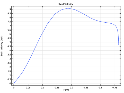
In the associated text field, type Swirl velocity (m/s).
|
|
1
|
|
2
|
|
1
|
|
2
|
|
3
|
|
4
|
|
5
|
|
6
|
|
7
|