|
|
|
|
1
|
|
2
|
In the Select Physics tree, select Electrochemistry>Tertiary Current Distribution, Nernst-Planck>Tertiary, Supporting Electrolyte (tcd).
|
|
3
|
Click Add.
|
|
4
|
|
5
|
In the Concentrations table, enter the following settings:
|
|
6
|
|
7
|
Click Add.
|
|
8
|
Click
|
|
9
|
In the Select Study tree, select Preset Studies for Selected Physics Interfaces>Tertiary Current Distribution, Nernst-Planck>Time Dependent with Initialization.
|
|
10
|
Click
|
|
1
|
|
2
|
|
3
|
|
4
|
Browse to the model’s Application Libraries folder and double-click the file znbr_flow_battery_parameters.txt.
|
|
1
|
|
2
|
|
3
|
|
4
|
|
5
|
Click to expand the Layers section. In the table, enter the following settings:
|
|
6
|
|
7
|
|
8
|
|
1
|
|
2
|
|
1
|
|
2
|
|
1
|
|
2
|
|
1
|
|
2
|
|
3
|
|
1
|
|
2
|
|
3
|
|
1
|
In the Model Builder window, under Component 1 (comp1) right-click Tertiary Current Distribution, Nernst-Planck (tcd) and choose Separator.
|
|
2
|
|
3
|
|
4
|
|
5
|
Locate the Electrolyte Current Conduction section. From the σl list, choose User defined. In the associated text field, type sigmal.
|
|
6
|
|
1
|
|
2
|
In the Settings window for Porous Electrode, type Porous Electrode - Negative in the Label text field.
|
|
3
|
|
4
|
|
5
|
Locate the Electrolyte Current Conduction section. From the σl list, choose User defined. In the associated text field, type sigmal.
|
|
6
|
Locate the Electrode Current Conduction section. From the σs list, choose User defined. In the associated text field, type sigmas_cf.
|
|
7
|
|
8
|
|
1
|
|
2
|
In the Settings window for Porous Electrode Reaction, locate the Stoichiometric Coefficients section.
|
|
3
|
|
4
|
|
5
|
|
6
|
|
7
|
|
1
|
|
2
|
In the Settings window for Porous Electrode, type Porous Electrode - Positive in the Label text field.
|
|
3
|
|
4
|
|
5
|
|
6
|
Locate the Electrolyte Current Conduction section. From the σl list, choose User defined. In the associated text field, type sigmal.
|
|
7
|
Locate the Electrode Current Conduction section. From the σs list, choose User defined. In the associated text field, type sigmas_cf.
|
|
8
|
|
9
|
|
1
|
|
2
|
In the Settings window for Porous Electrode Reaction, locate the Stoichiometric Coefficients section.
|
|
3
|
|
4
|
|
5
|
|
6
|
|
7
|
|
8
|
|
1
|
|
1
|
|
3
|
|
4
|
|
5
|
|
6
|
|
1
|
|
1
|
|
2
|
|
3
|
|
4
|
|
5
|
|
6
|
Locate the Electrode Kinetics section. From the Kinetics expression type list, choose Fast irreversible electrode reaction.
|
|
1
|
|
2
|
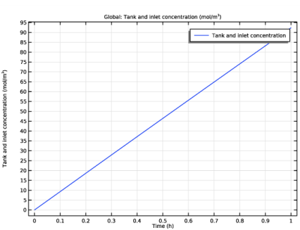
In the Settings window for Global ODEs and DAEs, type Global ODEs and DAEs - Tank Model in the Label text field.
|
|
1
|
In the Model Builder window, under Component 1 (comp1)>Global ODEs and DAEs - Tank Model (ge) click Global Equations 1.
|
|
2
|
|
3
|
|
4
|
Browse to the model’s Application Libraries folder and double-click the file znbr_flow_battery_global_equation.txt.
|
|
1
|
|
2
|
|
3
|
|
4
|
|
5
|
|
1
|
In the Model Builder window, under Component 1 (comp1)>Global ODEs and DAEs - Tank Model (ge) click Global Equations 1.
|
|
2
|
|
3
|
|
4
|
|
5
|
Click
|
|
6
|
|
7
|
Click OK.
|
|
8
|
|
9
|
|
10
|
In the Source term quantity table, enter the following settings:
|
|
1
|
In the Model Builder window, under Component 1 (comp1) click Tertiary Current Distribution, Nernst-Planck (tcd).
|
|
1
|
|
2
|
|
3
|
|
4
|
|
5
|
|
1
|
|
2
|
|
3
|
|
1
|
|
2
|
|
3
|
|
1
|
|
2
|
|
3
|
|
4
|
|
5
|
|
1
|
|
3
|
|
4
|
|
5
|
|
6
|
|
7
|
|
8
|
|
1
|
|
3
|
|
1
|
|
3
|
|
4
|
|
5
|
|
1
|
|
2
|
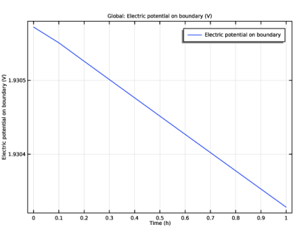
In the Settings window for Global Variable Probe, click Replace Expression in the upper-right corner of the Expression section. From the menu, choose Component 1 (comp1)>Tertiary Current Distribution, Nernst-Planck>tcd.phis0_ec1 - Electric potential on boundary - V.
|
|
1
|
|
2
|
|
3
|
|
4
|
|
1
|
|
2
|
|
3
|
|
4
|
|
1
|
|
1
|
|
2
|
|
1
|
|
2
|
|
1
|
In the Model Builder window, under Component 1 (comp1)>Tertiary Current Distribution, Nernst-Planck (tcd) click Porous Electrode - Negative.
|
|
2
|
In the Settings window for Porous Electrode, click to expand the Dissolving-Depositing Species section.
|
|
3
|
Click
|
|
1
|
|
2
|
In the Settings window for Porous Electrode Reaction, locate the Stoichiometric Coefficients section.
|
|
3
|
In the Stoichiometric coefficients for dissolving-depositing species: table, enter the following settings:
|
|
1
|
|
2
|
|
3
|
|
4
|
|
5
|
|
6
|
|
1
|
In the Model Builder window, under Component 1 (comp1)>Tertiary Current Distribution, Nernst-Planck (tcd) click Electrode Current 1.
|
|
2
|
|
3
|
|
1
|
In the Model Builder window, under Study 1 right-click Solver Configurations and choose Delete Configurations.
|
|
1
|
|
2
|
|
3
|
Click
|
|
1
|
|
2
|
|
3
|
Click
|
|
4
|
|
5
|
Click Replace.
|
|
1
|
|
2
|
|
3
|
Right-click Study 1>Solver Configurations>Solution 1 (sol1)>Time-Dependent Solver 1 and choose Stop Condition.
|
|
4
|
|
5
|
Click
|
|
7
|
|
8
|
|
1
|
|
2
|
|
3
|
|
4
|
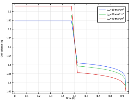
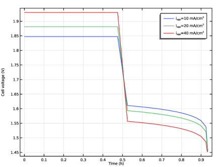
In the associated text field, type Cell voltage (V).
|
|
1
|
|
2
|
|
3
|
|
4
|
|
5
|
|
1
|
|
2
|
|
3
|
|
1
|
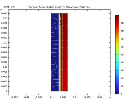
In the Model Builder window, expand the Results>Bromine Concentration node, then click Streamline 1.
|
|
2
|
|
3
|
|
4
|
Locate the Streamline Positioning section. From the Positioning list, choose On selected boundaries.
|
|
5
|
|
6
|
|
1
|
|
2
|
|
3
|
|
4
|
|
5
|
|
1
|
|
2
|
|
1
|
|
2
|
|
3
|
|
4
|
|
5
|
|
1
|
|
2
|
|
3
|
|
1
|
|
2
|
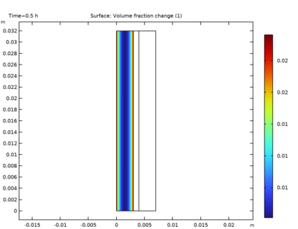
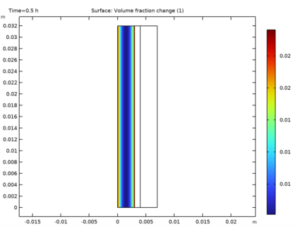
In the Settings window for 2D Plot Group, type Deposited Zinc Volume Fraction in the Label text field.
|
|
1
|
|
2
|
In the Settings window for Surface, click Replace Expression in the upper-right corner of the Expression section. From the menu, choose Component 1 (comp1)>Tertiary Current Distribution, Nernst-Planck>Dissolving-depositing species>tcd.deltaeps_pce1_Zn - Volume fraction change.
|
|
1
|
|
2
|
|
3
|
|
4
|
|
5
|
|
6
|