PDF

Primary Current Distribution in a Lead-Acid Battery Grid Electrode
Introduction
This example demonstrates the use of the Primary Current Distribution interface for modeling current distributions in electrochemical cells.
In primary current distribution, the potential losses due to electrode kinetics and mass transport are assumed to be negligible, and ohmic losses are govern the current distribution in the cell. Here you investigate primary current distribution in a positive lead-acid battery grid electrode during a high load (100 A) discharge.
In a traditional lead-acid electrode, the porous electrode is supported by a metal grid that also provides electronic conduction throughout the electrode. Optimizing the design of the grid leads to increased performance and lifetime as well as reduced weight (Ref. 1).
Model Definition
The half-cell geometry consists of a grid and a lug of the same metal material, a matrix of porous electrodes residing within the grid, and an electrolyte domain. The geometry is shown in Figure 1.
Figure 1: Modeled geometry
The Primary Current Distribution interface is used to model the current distribution in the half cell. The potential in the electrolyte is set to zero at the external boundary that is parallel to the grid. A discharge current of 100 A is applied to the end of the lug. Isolation is used for all other boundaries.
The equilibrium potential for the positive electrode reaction versus a reversible hydrogen electrode (RHE) is used to relate the electrode to the electrolyte phase potential:
The above condition is applied as a constraint in the porous electrode domains.
The problem is solved using a Stationary study.
Results and Discussion
Figure 2 shows the electrolyte potential in the electrolyte and the porous electrode domains. The potential drop is highest, roughly 0.2 V, in the area close to the lug.
Figure 2: Electrolyte potential in the electrolyte and porous electrodes.
Figure 3 shows the potential in the grid and the lug. The potential difference between the corner of the grid closest to the lug and the far end corner is about 0.15 V.
Figure 3: Electric potential in the grid and the lug.
Finally, the current density distribution in the electrolyte symmetry plane is plotted in Figure 4. The currents are about twice as high in the active region closest to the lug compared to the opposite corner of the cell.
In this case an improvement of the battery performance would be possible by making the frame of the grid thicker toward the lug corner, thereby achieving a more uniform current distribution.
Figure 4: Electrolyte current density at the half-cell boundary.
Reference
1. K. Yamada, K-I. Maeda, K. Sasaki, and T. Hirasawa “Computer-aided optimization of grid design for high-power lead-acid batteries,” J. Power Sources, selected papers from the Ninth European Lead Battery Conference, vol. 144, no. 2, pp. 352–357, 2005.
Application Library path: Battery_Design_Module/Batteries,_General/primary_cd_grid
Modeling Instructions
From the File menu, choose New.
New
In the New window, click  Model Wizard.
Model Wizard
1
In the Model Wizard window, click  3D.
2
In the Select Physics tree, select Electrochemistry>Primary and Secondary Current Distribution>Primary Current Distribution (cd).
3
Click Add.
4
Click  Study.
5
In the Select Study tree, select General Studies>Stationary.
6
Global Definitions
Parameters 1
1
In the Model Builder window, under Global Definitions click Parameters 1.
2
In the Settings window for Parameters, locate the Parameters section.
3
Click  Load from File.
4
Geometry 1
Start building the geometry using a work plane representing the electrode grid plane.
Work Plane 1 (wp1)
1
In the Geometry toolbar, click  Work Plane.
2
In the Settings window for Work Plane, locate the Plane Definition section.
3
From the Plane list, choose xz-plane.
4
Click  Show Work Plane.
Work Plane 1 (wp1)>Rectangle 1 (r1)
1
In the Work Plane toolbar, click  Rectangle.
2
In the Settings window for Rectangle, locate the Size and Shape section.
3
In the Width text field, type W.
4
In the Height text field, type H.
5
Click  Build Selected.
Work Plane 1 (wp1)>Plane Geometry
Draw one porous electrode section, then use it to create an array of porous electrodes.
Work Plane 1 (wp1)>Rectangle 2 (r2)
1
In the Work Plane toolbar, click  Rectangle.
2
In the Settings window for Rectangle, locate the Size and Shape section.
3
In the Width text field, type W_porous.
4
In the Height text field, type H_porous.
5
Locate the Position section. In the xw text field, type s_frame.
6
In the yw text field, type s_frame.
Work Plane 1 (wp1)>Array 1 (arr1)
1
In the Work Plane toolbar, click  Transforms and choose Array.
2
3
In the Settings window for Array, locate the Size section.
4
In the xw size text field, type N_x.
5
In the yw size text field, type N_z.
6
Locate the Displacement section. In the xw text field, type W_porous+s_grid.
7
In the yw text field, type H_porous+s_grid.
8
Click  Build Selected.
Work Plane 1 (wp1)>Plane Geometry
Draw the lug as an additional rectangle. It has the same thickness as the electrode.
Work Plane 1 (wp1)>Rectangle 3 (r3)
1
In the Work Plane toolbar, click  Rectangle.
2
In the Settings window for Rectangle, locate the Size and Shape section.
3
In the Width text field, type W_lug.
4
In the Height text field, type H_lug.
5
Locate the Position section. In the xw text field, type W-s_frame-W_lug.
6
In the yw text field, type H.
7
Click  Build Selected.
8
Click the  Zoom Extents button in the Graphics toolbar.
Extrude 1 (ext1)
1
In the Model Builder window, under Component 1 (comp1)>Geometry 1 right-click Work Plane 1 (wp1) and choose Extrude.
2
In the Settings window for Extrude, locate the Distances section.
3
4
Click  Build Selected.
Electrolyte
Finalize the geometry by drawing the electrolyte domain.
1
In the Geometry toolbar, click  Block.
2
In the Settings window for Block, locate the Size and Shape section.
3
In the Width text field, type W.
4
In the Depth text field, type d_electrolyte.
5
In the Height text field, type H.
6
Locate the Selections of Resulting Entities section. Select the Resulting objects selection check box.
7
Right-click Block 1 (blk1) and choose Rename.
8
In the Rename Block dialog box, type Electrolyte in the New label text field.
9
10
In the Settings window for Block, click  Build All Objects.
11
Click the  Zoom Extents button in the Graphics toolbar.
The completed geometry should look as shown in the following figure:
Definitions
Create a selection for the union of the grid and lug domains to facilitate setting up the model.
Grid + Lug
1
In the Definitions toolbar, click  Explicit.
2
3
Right-click Explicit 1 and choose Rename.
4
In the Rename Explicit dialog box, type Grid + Lug in the New label text field.
5
Porous Electrodes
Use a Complement selection to select the porous electrodes.
1
In the Definitions toolbar, click  Complement.
2
In the Settings window for Complement, locate the Input Entities section.
3
Under Selections to invert, click  Add.
4
In the Add dialog box, in the Selections to invert list, choose Grid + Lug and Electrolyte.
5
6
Right-click Complement 1 and choose Rename.
7
In the Rename Complement dialog box, type Porous Electrodes in the New label text field.
8
Primary Current Distribution (cd)
Electrode 1
1
In the Model Builder window, under Component 1 (comp1) right-click Primary Current Distribution (cd) and choose Electrode.
2
In the Settings window for Electrode, locate the Domain Selection section.
3
From the Selection list, choose Grid + Lug.
4
Locate the Electrode section. From the σs list, choose User defined. In the associated text field, type sigma_metal.
Porous Electrode 1
1
In the Physics toolbar, click  Domains and choose Porous Electrode.
2
In the Settings window for Porous Electrode, locate the Domain Selection section.
3
From the Selection list, choose Porous Electrodes.
4
Locate the Electrolyte Current Conduction section. From the σl list, choose User defined. In the associated text field, type sigma_electrolyte.
5
Locate the Electrode Current Conduction section. From the σs list, choose User defined. In the associated text field, type sigma_porous.
Porous Electrode Reaction 1
1
In the Model Builder window, click Porous Electrode Reaction 1.
2
In the Settings window for Porous Electrode Reaction, locate the Equilibrium Potential section.
3
In the Eeq text field, type 1.7.
Electrolyte 1
1
In the Model Builder window, under Component 1 (comp1)>Primary Current Distribution (cd) click Electrolyte 1.
2
In the Settings window for Electrolyte, locate the Electrolyte section.
3
From the σl list, choose User defined. In the associated text field, type sigma_electrolyte.
Electrolyte Potential 1
1
In the Physics toolbar, click  Boundaries and choose Electrolyte Potential.
2
Electrode Current 1
1
In the Physics toolbar, click  Boundaries and choose Electrode Current.
2
3
In the Settings window for Electrode Current, locate the Electrode Current section.
4
In the Is,total text field, type -100.
Definitions
The highest gradients in the model are to be expected at the edges between the porous electrode and the electrolyte. Create a selection of these edges to use later when setting up the mesh.
Adjacent 1
1
In the Definitions toolbar, click  Adjacent.
2
In the Settings window for Adjacent, locate the Input Entities section.
3
Under Input selections, click  Add.
4
In the Add dialog box, select Porous Electrodes in the Input selections list.
5
6
In the Settings window for Adjacent, locate the Output Entities section.
7
From the Geometric entity level list, choose Adjacent edges.
Adjacent 2
1
In the Definitions toolbar, click  Adjacent.
2
In the Settings window for Adjacent, locate the Input Entities section.
3
Under Input selections, click  Add.
4
In the Add dialog box, select Electrolyte in the Input selections list.
5
6
In the Settings window for Adjacent, locate the Output Entities section.
7
From the Geometric entity level list, choose Adjacent edges.
Intersection 1
1
In the Definitions toolbar, click  Intersection.
2
In the Settings window for Intersection, locate the Geometric Entity Level section.
3
From the Level list, choose Edge.
4
Locate the Input Entities section. Under Selections to intersect, click  Add.
5
In the Add dialog box, in the Selections to intersect list, choose Adjacent 1 and Adjacent 2.
6
Mesh 1
Edge 1
1
In the Mesh toolbar, click  Boundary and choose Edge.
2
In the Settings window for Edge, locate the Edge Selection section.
3
From the Selection list, choose Intersection 1.
Size 1
1
Right-click Edge 1 and choose Size.
2
In the Settings window for Size, locate the Element Size section.
3
Click the Custom button.
4
Locate the Element Size Parameters section. Select the Maximum element size check box.
5
Free Tetrahedral 1
1
In the Mesh toolbar, click  Free Tetrahedral.
2
In the Model Builder window, right-click Mesh 1 and choose Build All.
Study 1
In the Home toolbar, click  Compute.
Results
Electrolyte Potential (cd)
The electrolyte potential (Figure 2) and electrode potential versus ground (Figure 3) are plotted by default.
Electrolyte Current Density at the Half-cell Boundary
To create Figure 4, do the following steps.
1
In the Home toolbar, click  Add Plot Group and choose 3D Plot Group.
2
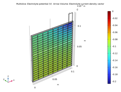
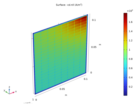
In the Settings window for 3D Plot Group, type Electrolyte Current Density at the Half-cell Boundary in the Label text field.
3
Locate the Plot Settings section. Clear the Plot dataset edges check box.
Surface 1
1
Right-click Electrolyte Current Density at the Half-cell Boundary and choose Surface.
2
In the Settings window for Surface, locate the Expression section.
3
In the Expression text field, type -cd.nIl.
Selection 1
1
Right-click Surface 1 and choose Selection.
2
3
In the Electrolyte Current Density at the Half-cell Boundary toolbar, click  Plot.