Modeling Impedance in the Lithium-Ion Battery

Electrochemical impedance spectroscopy (EIS) is a valuable method to investigate electrochemical systems such as batteries. For a battery, where potential perturbations of varying frequency are applied on an electrode, the impedance response gives insight into several battery properties and processes. At high frequencies, short time-scale processes such as capacitance, electrochemical reactions, and local resistances affect the impedance. On the other hand, at low frequencies, diffusion in the electrolyte and active material particles (that is, large time-scale processes) contribute to the impedance.

This example simulates the impedance of a full lithium-ion battery cell using the Lithium-Ion Battery interface with an AC Impedance Stationary study. The model also reproduces to the results by Abraham and others (Ref. 1) for sinusoidal potential perturbations between 10 mHz to 1 kHz after model fitting using the Parameter Estimation study step.

This tutorial model requires the Optimization Module.

Model Definition

The model consists of the following components:

•

Negative porous electrode: LTO (Li4Ti5O12) active material, electronic conductor, and filler.

•

Separator: Celgard 2325

•

Positive porous electrode: NCA (LiNi0.08Co0.15Al0.05O2) active material, electronic conductor, and filler.

•

Electrolyte: 1.2 M LiPF6 in EC:EMC (3:7 by weight)

A 1D model with three domains of different thickness is used: a 115 μm negative electrode, a 50 μm separator, and a 35 μm positive electrode. The model is set up in a similar fashion as the 1D Isothermal Lithium-Ion Battery, but with double-layer capacitances on the active electrode materials and on the electronic conductor in the positive electrode. The model approach using an additional double-layer at the electronic conductor has, for example, been used by Brown and others (Ref. 2) to describe experimental EIS spectra measured between 1 mHz and 1 kHz on NCA electrodes.

An AC Stationary Impedance study is used to solve the problem, implying that all variables are shifted from being time dependent to frequency dependent, as illustrated with the following expression:

where n is the variable and subscript 0 denotes the initial value around which the perturbation takes place and tilde the complex perturbation. Furthermore, i is the imaginary unit, f the frequency, and t the time.

The boundary of the positive electrode current-collector is set to a sinusoidal perturbation with a 10 mV amplitude and the boundary of the negative electrode current-collector fixed to 0 V, that is, ground.

The cell impedance, Z (SI unit: Ω·m2), is calculated at the boundary of the positive electrode current-collector as follows:

where

(SI unit: V) is the potential, n the boundary normal and Is (SI unit: Am−2) the current density in the solid. (Note that the lindev operator is used in the model file in order to use the perturbing values of the variables in the evaluation.)

Subtracting the reference electrode potential from the solid potential in the numerator enables the analysis of the impedance of the NCA positive electrode versus the reference electrode, thus separating the contribution of each electrode to the impedance. The LTO impedance versus the reference is consequently given by the difference between the cell impedance and NCA impedance versus the reference.

The model is computed for frequencies between 10 mHz and 1 kHz. This range is common in EIS to minimize any errors from experimental interference (for example, Ref. 2).

Optimization

The model is initially solved for the presented experimental set-up (Ref. 1) with the aid of parameters given in Ref. 2. However, since the simulated impedance deviates to a large extent from the experiments, an optimization is performed using the Global Least-Squares Objective feature in the Optimization interface. This feature is set to minimize the least-squares error between the simulated and measured NCA impedance versus the reference electrode through variation of some control parameters. These parameters are given in Table 1.

Table 1: control parameters with bounds For a Cell voltage of 2.30V.
Control parameters	Initial value	Bounds
Exchange current density NCA	1 Am-2	Lower: 1 Am-2 Upper: 6 Am-2
Double-layer capacitance NCA	5·10-1 Fm-2	Lower: 1·10-1 Fm-2 Upper: 9·10-1 Fm-2
Film resistance NCA	1·10-3 Ωm2	Lower: 1·10-6 Ωm2 Upper: 5·10-3 Ωm2
Volumetric double-layer capacitance positive electronic conductor	5·105 Fm-3	Lower: 1·105 Fm-3 Upper: 1·106 Fm-3

The first three parameters have bounds selected as anticipated by the information given by Abraham and others (Ref. 1). The last parameter depend on the size of the electronic conductor particles. It is also common to run parametric sweeps before selecting control parameters and to narrow down the bounds. Normally the optimization time is reduced and the optimization accuracy is improved when few control parameters and narrow bound intervals are selected.

Study settings

The problem is solved with an AC Impedance, Initial Values study. The optimization solver is set up by adding an Optimization node to the study and selecting the SNOPT method with the numeric gradient method.

Results and Discussion

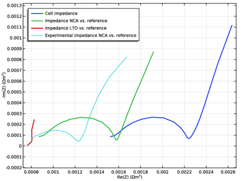
Simulated and experimental Nyquist spectra from the LTO/NCA cell at 2.30 V are displayed in Figure 1. The simulation utilizes the parameters from Ref. 2. Characteristic semi-circles and low-frequency tails are seen. The largest contribution to the cell impedance is in the positive NCA electrode. The difference between the experimental and simulated impedance spectra of the NCA electrode versus reference is evident: The simulation shows one large semi-circle and an indication of another semi-circle at high frequencies. The experimental spectrum has a smaller depressed (elongated) semi-circle.

Figure 1: Simulated and experimental Nyquist spectra for 10 mHz to 1 kHz. Parameters taken from Ref. 2.

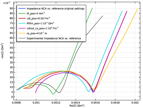
Since the difference is most prominent in the semi-circle frequency region (that is, mid-high frequencies) mainly the parameters describing short time-scale processes do not fit the experiments. Four of these parameters are investigated with a parametric sweep to determine their impact on the impedance. The sweep is shown in Figure 2.

Figure 2: Nyquist plots when testing the impact of five parameters for 10 mHz to 1 kHz.

As a comparison, the sweep also includes variation of the radius of the positive electrode material particles, mainly affecting the large time-scale process of diffusion in the particles. Its impact is therefore more evident at lower frequencies. This is seen in Figure 2, where both the angle and shape of the low-frequency tail change. The results also show that the parameters describing large time-scale processes seem to be quite accurate in the model.

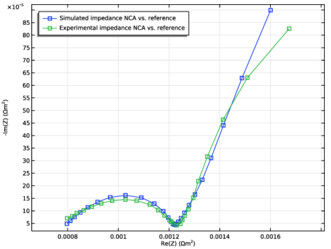
These findings are consistent with the observations by Abraham and others (Ref. 1) indicating that the electrochemical reaction is less limited in their electrodes. With this input Table 1 is set up and the optimization is run. The resulting spectra are shown in Figure 3.

Figure 3: Nyquist spectra with optimized parameters for 10 mHz to 1 kHz. Squares denote the data points used in the optimization.

The simulated and experimental spectra for NCA versus reference are now seen to overlap well. The optimized control parameters are tabulated in Table 2.

Table 2: Change of control parameters After optimization.
Control Parameters	Optimized Value
Exchange current density NCA	2.5 Am-2
Double-layer capacitance NCA	4.1·10-1 Fm-2
Film resistance NCA	1·10-6 Ωm2
Volumetric double-layer capacitance positive electronic conductor	5.6·105 Fm-3

References

1. D.P. Abraham, S. Kawauchi, and D.W. Dees, “Modeling the impedance versus voltage characteristics of LiNi0.08Co0.15Al0.05O2,” Electrochim. Acta, vol. 53, pp. 2121–2129, 2008.

2. S. Brown, N. Mellgren, M. Vynnycky, and G. Lindbergh, “Impedance as a Tool for Investigating Aging in Lithium-Ion Porous Electrodes. II. Positive Electrode Examination,” J. Electrochem. Soc, vol. 155, p. A320, 2008.

Battery_Design_Module/Batteries,_Lithium-Ion/li_battery_impedance

Modeling Instructions

From the menu, choose .

New

In the window, click

Model Wizard

In the window, click

In the tree, select .

Click .

Click

In the tree, select .

Click

Global Definitions

Load parameters from a text file

Parameters 1

In the window, under click .

In the window for , locate the section.

Click

Browse to the model’s Application Libraries folder and double-click the file li_battery_impedance_parameters.txt.

Definitions

The impedance is calculated using variables defined in a text file. It is defined at the rightmost boundary versus ground (at the leftmost boundary) or a reference electrode. The lindev operator explicitly evaluates the deviation from the stationary solution in the perturbed solution.

Variables 1

In the window, under right-click and choose .

In the window for , locate the section.

Click

Browse to the model’s Application Libraries folder and double-click the file li_battery_impedance_variables.txt.

Geometry 1

Interval 1 (i1)

In the window, under right-click and choose .

In the window for , locate the section.

In the table, enter the following settings:


Coordinates (m)
0
L_neg

Interval 2 (i2)

In the window, right-click and choose .

In the window for , locate the section.

From the list, choose .

In the text field, type L_neg.

In the table, enter the following settings:


Lengths (m)
L_sep

Interval 3 (i3)

Right-click and choose .

In the window for , locate the section.

From the list, choose .

In the text field, type L_neg+L_sep.

In the table, enter the following settings:


Lengths (m)
L_pos

Click

Click the

button in the toolbar.

Add Material

The cell materials are available in the Battery Material Library.

In the toolbar, click

to open the window.

Go to the window.

In the tree, select .

Click in the window toolbar.

In the tree, select .

Click in the window toolbar.

In the tree, select .

Click in the window toolbar.

In the toolbar, click

to close the window.

Definitions

Use a domain point probe to retrieve the potential in the middle of the separator where the reference electrode is located.

Reference Electrode (RE) Probe

In the toolbar, click

and choose .

In the window for , type Reference Electrode (RE) Probe in the text field.

Locate the section. In row , set to L_neg+L_sep/2.

Point Probe Expression 1 (ppb1)

In the window, expand the node, then click .

In the window for , type RE_phi in the text field.

Integration 1 (intop1)

In the toolbar, click

and choose .

In the window for , locate the section.

From the list, choose .

Select Boundary 4 only.

Lithium-Ion Battery (liion)

Set up the model with a negative and a positive porous electrode with a separator in between. Double layers exist on both active materials.

Porous Electrode 1

In the window, under right-click and choose .

Select Domain 1 only.

In the window for , locate the section.

From the list, choose .

Click to expand the section. From the list, choose .

In the Rfilm text field, type Rfilm_neg.

Locate the section. In the εs text field, type epss_neg.

In the εl text field, type epsl_neg.

Locate the section. From the list, choose . In the fl text field, type epsl_neg^brugl_neg.

From the list, choose . In the fDl text field, type epsl_neg^brugl_neg.

Particle Intercalation 1

In the window, click .

In the window for , locate the section.

From the list, choose .

Locate the section. In the cs,init text field, type mat2.elpot.cEeqref*soc0_neg.

Locate the section. In the rp text field, type rp_neg.

Porous Electrode Reaction 1

In the window, click .

In the window for , locate the section.

From the list, choose .

Locate the section. In the i0,ref(T) text field, type i0ref_neg.

Porous Electrode 1

In the window, click .

Porous Matrix Double Layer Capacitance 1

In the toolbar, click

and choose .

In the window for , locate the section.

In the Cdl text field, type cdl_neg.

Porous Electrode 2

In the toolbar, click

and choose .

Select Domain 3 only.

In the window for , locate the section.

From the list, choose .

Locate the section. From the list, choose .

In the Rfilm text field, type Rfilm_pos.

Locate the section. In the εs text field, type epss_pos.

In the εl text field, type epsl_pos.

Locate the section. From the list, choose . In the fl text field, type epsl_pos^brugl_pos.

From the list, choose . In the fDl text field, type epsl_pos^brugl_pos.

Particle Intercalation 1

In the window, click .

In the window for , locate the section.

From the list, choose .

Locate the section. In the cs,init text field, type mat3.elpot.cEeqref*soc0_pos.

Locate the section. In the rp text field, type rp_pos.

Porous Electrode Reaction 1

In the window, click .

In the window for , locate the section.

From the list, choose .

Locate the section. From the list, choose .

In the i0 text field, type i0_pos.

Locate the section. From the list, choose . In the av text field, type as_pos.

Porous Electrode 2

In the window, click .

Porous Matrix Double Layer Capacitance 1

In the toolbar, click

and choose .

In the window for , locate the section.

In the Cdl text field, type cdl_pos.

From the list, choose . In the av,dl text field, type as_pos.

Separator 1

In the toolbar, click

and choose .

Select Domain 2 only.

In the window for , locate the section.

In the εl text field, type epsl_sep.

Locate the section. From the list, choose . In the fl text field, type epsl_sep^brugl_sep.

From the list, choose . In the fDl text field, type epsl_sep^brugl_sep.

Initial Values 1

In the window, click .

In the window for , locate the section.

In the list, select .

Locate the section. In the phil text field, type -mat2.elpot.Eeq_int1(soc0_neg).

In the cl text field, type cl_init.

Initial Values 2

In the toolbar, click

and choose .

Select Domain 3 only.

In the window for , locate the section.

In the phil text field, type -mat2.elpot.Eeq_int1(soc0_neg).

In the cl text field, type cl_init.

In the phis text field, type mat3.elpot.Eeq_int1(soc0_pos)-mat2.elpot.Eeq_int1(soc0_neg).

Electric Ground 1

Select ground on the current collector of the negative LTO electrode. Set a 10 mV perturbation around the cell voltage of 2.30 V.

In the toolbar, click

and choose .

Select Boundary 1 only.

Electric Potential 1

In the toolbar, click

and choose .

Select Boundary 4 only.

In the window for , locate the section.

In the φs,bnd text field, type E_cell_init.

Harmonic Perturbation 1

In the toolbar, click

and choose .

In the window for , locate the section.

In the Δφs text field, type E_pert.

Additional Porous Electrode Material 1

Add an Additional Porous Electrode Material feature to model the electronic conductor in NCA.

In the toolbar, click

and choose .

Select Domain 3 only.

In the window for , locate the section.

From the list, choose .

Porous Electrode Reaction 1

No electrochemical reaction takes place on the electronic conductor, but a double layer capacitance exists.

In the window, right-click and choose .

Additional Porous Electrode Material 1

In the window, click .

Porous Matrix Double Layer Capacitance 1

In the toolbar, click

and choose .

In the window for , locate the section.

In the Cdl text field, type 1[F/m^2].

From the list, choose . In the av,dl text field, type cdlvol_cs_pos/1[F/m^2].

Mesh 1

In the window, under click .

In the window for , locate the section.

From the list, choose .

Size

In the window, under click .

In the window for , locate the section.

Click the button.

Locate the section. In the text field, type 1e-5.

Size 1

In the window, click .

Select Domains 2 and 3 only.

In the window for , locate the section.

Click the button.

Locate the section. Select the check box.

In the associated text field, type 1e-6.

Size 2

In the window, click .

Select Boundaries 2–4 only.

In the window for , locate the section.

Click the button.

Locate the section. Select the check box.

In the associated text field, type 5E-7.

Study 1

Solve the model for frequencies between 10 mHz and 1 kHz.

In the window, click .

In the window for , locate the section.

Clear the check box.

Step 1: Frequency Domain Perturbation

In the window, under click .

In the window for , locate the section.

In the text field, type 10^{range(-2,0.2,3)}.

In the toolbar, click

Study 1

Solution 1 (sol1)

Save the solution of the nonoptimized impedance results.

In the window, under right-click and choose .

Expand the node.

Not optimized

In the window, expand the node, then click .

In the window for , type Not optimized in the text field.

Results

Follow these steps to generate Figure 1:

Start by loading experimental data of real and imaginary impedance into a table for plotting purposes. Organize the tables by naming them.

Experimental Impedance Table

In the toolbar, click

In the window for , type Experimental Impedance Table in the text field.

Locate the section. Click .

Browse to the model’s Application Libraries folder and double-click the file li_battery_impedance_Zexp.csv.

Reference Electrode (RE) Probe Table

In the window, under click .

In the window for , type Reference Electrode (RE) Probe Table in the text field.

Reference Electrode (RE) Potential Probe Plot

In the window, under click .

In the window for , type Reference Electrode (RE) Potential Probe Plot in the text field.

Nyquist plots

In the toolbar, click

In the window for , type Nyquist plots in the text field.

Click to expand the section. Locate the section. From the list, choose .

Locate the section. From the list, choose .

Locate the section. Select the check box.

In the associated text field, type Re(Z) ([Omega]m<sup>2</sup>).

Select the check box.

In the associated text field, type -Im(Z) ([Omega]m<sup>2</sup>).

Cell impedance

Right-click and choose .

In the window for , type Cell impedance in the text field.

Select Boundary 4 only.

Locate the section. In the text field, type -imag(Z_ground).

Locate the section. From the list, choose .

In the text field, type real(Z_ground).

Click to expand the section. In the text field, type 2.

Click to expand the section. Select the check box.

From the list, choose .

In the table, enter the following settings:


Legends
Cell impedance

Impedance NCA vs. reference

Right-click and choose .

In the window for , type Impedance NCA vs. reference in the text field.

Locate the section. In the text field, type -imag(Z_ref_NCA).

Click to expand the section. From the list, choose .

Locate the section. In the text field, type real(Z_ref_NCA).

Locate the section. In the table, enter the following settings:


Legends
Impedance NCA vs. reference

Impedance LTO vs. reference

Right-click and choose .

In the window for , type Impedance LTO vs. reference in the text field.

Locate the section. In the text field, type -imag(Z_ref_LTO).

Locate the section. In the text field, type real(Z_ref_LTO).

Locate the section. In the table, enter the following settings:


Legends
Impedance LTO vs. reference

Experimental impedance NCA vs. reference

In the window, right-click and choose .

The Table Graph plots the experimental data that was imported into the Experimental Impedance Table.

In the window for , type Experimental impedance NCA vs. reference in the text field.

Locate the section. From the list, choose .

From the list, choose .

In the list, select .

Click to expand the section. Select the check box.

From the list, choose .

In the table, enter the following settings:


Legends
Experimental impedance NCA vs. reference

Nyquist plots

In the window, click .

In the window for , locate the section.

From the list, choose .

Locate the section. Select the check box.

In the toolbar, click

Click the

button in the toolbar.

Study 1

Add a parametric sweep to investigate the impact four key parameters have on the impedance of NCA versus the reference and how it relates to the experimental measurements.

Parametric Sweep

In the toolbar, click

In the window for , locate the section.

Click

Browse to the model’s Application Libraries folder and double-click the file li_battery_impedance_parametric_sweep.txt.

In the toolbar, click

Parametric sweep

In the window, under click .

In the window for , type Parametric sweep in the text field.

Results

Nyquist plots parametric sweep

In the window, right-click and choose .

Rename the solution for the parametric sweep.

In the window for , type Nyquist plots parametric sweep in the text field.

Follow these steps to generate Figure 2:

Impedance NCA vs. reference

In the window, expand the node, then click .

In the window for , locate the section.

From the list, choose .

Locate the section. In the table, enter the following settings:


Legends
Impedance NCA vs. reference original settings
i0_pos=5 Am<sup>-2</sup>
cdl_pos=0.50 Fm<sup>-2</sup>
Rfilm_pos=1<sup>.</sup>10<sup>-5</sup> Ωm<sup>2</sup>
cdlvol_cs_pos=1<sup>.</sup>10<sup>4</sup> Fm<sup>-3</sup>
rp_pos=4<sup>.</sup>10<sup>-7</sup> m

Cell impedance

In the window, right-click and choose .

Impedance LTO vs. reference

In the window, right-click and choose .

Nyquist plots parametric sweep

In the window, click .

In the toolbar, click

Click the

button in the toolbar.

Add Study

In the toolbar, click

to open the window.

Go to the window.

Find the subsection. In the tree, select .

Click in the window toolbar.

In the toolbar, click

to close the window.

Study 2

In the window, click .

In the window for , locate the section.

Clear the check box.

Parameter Estimation

Select i0_pos, Rfilm_pos, cdl_pos, and cslvol_cs_pos as the four parameters to be optimized. The Optimization tolerance is set to 1e-4.

In the toolbar, click

and choose .

Import the experimental data in csv format for the impedance of the NCA electrode versus the reference.

In the window for , locate the section.

In the text field, type li_battery_impedance_Zexp.csv.

Click

Locate the section. In the table, enter the following settings:


Columns	Type	Settings
Column 1	Frequency	Frequency unit=Hz
Column 2	Value	Model expression=1, Name=col2, Weight=1
Column 3	Value	Model expression=1, Name=col3, Weight=1

The second column of the experimental data contains the global value real impedance.

In the table, click to select the cell at row number 2 and column number 3.

In the table, enter the following settings:


Columns	Type	Settings
Column 1	Frequency	Frequency unit=Hz
Column 2	Value	Model expression=1, Name=col2, Weight=1
Column 3	Value	Model expression=1, Name=col3, Weight=1

The third column of the experimental data contains the global value imaginary impedance.

In the table, click to select the cell at row number 2 and column number 3.

In the text field, type comp1.intop1(real(Z_ref_NCA)).

In the text field, type Real_impedance.

In the text field, type 1e6.

In the table, click to select the cell at row number 3 and column number 3.

In the table, enter the following settings:


Columns	Type	Settings
Column 1	Frequency	Frequency unit=Hz
Column 2	Value	Model expression=comp1.intop1(real(Z_ref_NCA)), Name=Real_impedance, Weight=1e6
Column 3	Value	Model expression=-comp1.intop1(imag(Z_ref_NCA)), Name=col3, Weight=1

In the text field, type -comp1.intop1(imag(Z_ref_NCA)).

In the text field, type Imaginary_impedance.

In the text field, type 1e6.

Locate the section. Click

four times.

In the table, enter the following settings:


Parameter name	Initial value	Scale	Lower bound	Upper bound
i0_pos (Exchange current density positive electrode)	1[A/m^2]	1	1	6
Rfilm_pos (Film resistance positive electrode)	1e-3[m^2/S]	1e-3	1e-6	5e-3
cdl_pos (Double layer capacitance positive electrode material)	0.5[F/m^2]	1	0.10	0.90
cdlvol_cs_pos (Volumetric capacitance of electronic conductor in positive electrode)	5e5[F/m^3]	1e5	1e5	1e6