
|
|
|
|
1
|
|
2
|
In the Select Physics tree, select Electrochemistry>Tertiary Current Distribution, Nernst-Planck>Tertiary, Water-Based with Electroneutrality (tcd).
|
|
3
|
Click Add.
|
|
4
|
Click
|
|
5
|
|
6
|
Click
|
|
1
|
|
2
|
|
3
|
|
4
|
Browse to the model’s Application Libraries folder and double-click the file electrochemical_capacitor_side_reactions_electrochemical_cell.txt.
|
|
5
|
|
1
|
|
2
|
|
3
|
|
4
|
Browse to the model’s Application Libraries folder and double-click the file electrochemical_capacitor_side_reactions_load_profile.txt.
|
|
1
|
|
2
|
In the Settings window for Parameters, type Parameters : Electrode Reactions in the Label text field.
|
|
3
|
|
4
|
Browse to the model’s Application Libraries folder and double-click the file electrochemical_capacitor_side_reactions_electrode_reactions.txt.
|
|
1
|
|
2
|
|
1
|
In the Model Builder window, expand the Component 1 (comp1)>Geometry 1>Interval 1 (i1) node, then click Interval 1 (i1).
|
|
2
|
|
3
|
|
1
|
In the Model Builder window, under Component 1 (comp1) click Tertiary Current Distribution, Nernst-Planck (tcd).
|
|
2
|
In the Settings window for Tertiary Current Distribution, Nernst-Planck, click to expand the Dependent Variables section.
|
|
3
|
|
4
|
In the Concentrations table, enter the following settings:
|
|
1
|
In the Model Builder window, under Component 1 (comp1)>Tertiary Current Distribution, Nernst-Planck (tcd) click Electrolyte 1.
|
|
2
|
|
3
|
|
4
|
|
5
|
|
6
|
|
7
|
|
8
|
|
1
|
In the Model Builder window, under Component 1 (comp1)>Tertiary Current Distribution, Nernst-Planck (tcd) click Initial Values 1.
|
|
2
|
|
3
|
|
4
|
|
5
|
|
1
|
|
2
|
|
3
|
|
4
|
|
5
|
Click OK.
|
|
6
|
|
7
|
|
8
|
|
9
|
|
10
|
|
1
|
|
2
|
|
3
|
|
4
|
|
5
|
Click OK.
|
|
6
|
|
7
|
|
8
|
|
9
|
|
10
|
|
11
|
|
1
|
|
2
|
In the Settings window for Porous Electrode, type Porous Electrode - H2 side in the Label text field.
|
|
3
|
|
4
|
|
5
|
Click OK.
|
|
6
|
|
7
|
|
8
|
|
9
|
|
10
|
|
11
|
|
12
|
|
13
|
Locate the Electrode Current Conduction section. From the σs list, choose User defined. In the associated text field, type sigma_s.
|
|
14
|
|
15
|
|
1
|
In the Model Builder window, under Component 1 (comp1)>Tertiary Current Distribution, Nernst-Planck (tcd)>Porous Electrode - H2 side click Porous Electrode Reaction 1.
|
|
2
|
In the Settings window for Porous Electrode Reaction, type Porous Electrode Reaction - HER in the Label text field.
|
|
3
|
|
4
|
|
5
|
|
6
|
|
7
|
|
1
|
|
2
|
In the Settings window for Porous Matrix Double Layer Capacitance, locate the Porous Matrix Double Layer Capacitance section.
|
|
3
|
|
4
|
|
5
|
|
6
|
|
1
|
|
2
|
In the Settings window for Porous Electrode, type Porous Electrode - O2 side in the Label text field.
|
|
3
|
|
4
|
|
5
|
|
6
|
Click OK.
|
|
1
|
In the Model Builder window, expand the Porous Electrode - O2 side node, then click Porous Electrode Reaction - HER.
|
|
2
|
In the Settings window for Porous Electrode Reaction, type Porous Electrode Reaction - OER in the Label text field.
|
|
3
|
|
4
|
|
5
|
|
6
|
|
7
|
|
1
|
|
2
|
In the Settings window for Internal Electrode Surface, type Internal Electrode Surface -ORR in the Label text field.
|
|
3
|
|
4
|
|
5
|
Click OK.
|
|
1
|
|
2
|
|
3
|
|
4
|
|
5
|
Locate the Equilibrium Potential section. From the Eeq list, choose User defined. Locate the Electrode Kinetics section. From the Kinetics expression type list, choose Fast irreversible electrode reaction.
|
|
6
|
|
1
|
|
2
|
|
3
|
|
4
|
|
6
|
|
1
|
In the Model Builder window, expand the Internal Electrode Surface -HOR node, then click Electrode Reaction 1.
|
|
2
|
|
3
|
|
4
|
|
5
|
|
6
|
|
1
|
|
2
|
|
3
|
|
4
|
|
5
|
Click OK.
|
|
1
|
|
2
|
|
3
|
|
4
|
|
5
|
Click OK.
|
|
6
|
|
7
|
|
8
|
|
9
|
|
10
|
|
11
|
|
12
|
|
13
|
|
14
|
|
1
|
|
2
|
|
3
|
|
4
|
|
5
|
Select the Description check box.
|
|
1
|
|
2
|
|
3
|
|
4
|
|
1
|
|
2
|
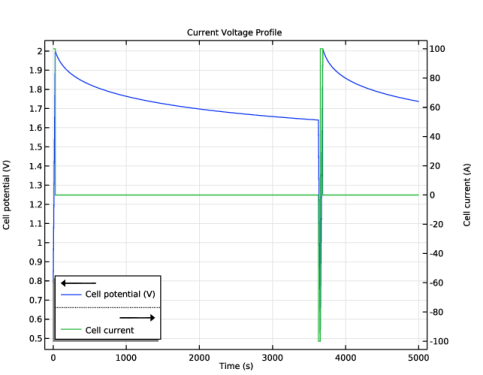
In the Settings window for Global Variable Probe, click Replace Expression in the upper-right corner of the Expression section. From the menu, choose Component 1 (comp1)>Tertiary Current Distribution, Nernst-Planck>Charge-Discharge Cycling 1>tcd.cdc1.phis0 - Cell potential - V.
|
|
3
|
|
1
|
|
2
|
|
3
|
|
1
|
|
2
|
|
3
|
|
4
|
|
1
|
|
2
|
|
1
|
|
2
|
In the Settings window for Study, type Study 1 : CC Charge with Rest Period in the Label text field.
|
|
3
|
|
1
|
In the Model Builder window, expand the Study 1 : CC Charge with Rest Period node, then click Step 1: Time Dependent.
|
|
2
|
|
3
|
|
1
|
|
2
|
|
3
|
Right-click Study 1 : CC Charge with Rest Period>Solver Configurations>Solution 1 (sol1)>Time-Dependent Solver 1 and choose Compute.
|
|
1
|
|
2
|
|
3
|
|
4
|
|
1
|
|
2
|
|
3
|
|
4
|
|
5
|
|
6
|
|
1
|
|
2
|
In the Settings window for Global, click Replace Expression in the upper-right corner of the y-Axis Data section. From the menu, choose Component 1 (comp1)>Tertiary Current Distribution, Nernst-Planck>Charge-Discharge Cycling 1>tcd.cdc1.Icell - Cell current - A.
|
|
3
|
|
1
|
|
2
|
|
3
|
|
4
|
|
5
|
|
6
|
|
1
|
|
2
|
|
3
|
|
4
|
|
5
|
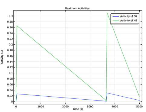
In the associated text field, type Activity (1).
|
|
1
|
|
2
|
|
3
|
|
1
|
|
2
|
|
3
|
|
4
|
|
5
|
|
1
|
|
2
|
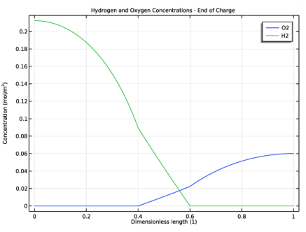
In the Settings window for 1D Plot Group, type Hydrogen and Oxygen Concentrations - End of Charge in the Label text field.
|
|
3
|
|
4
|
|
5
|
|
6
|
|
7
|
In the associated text field, type Dimensionless length (1).
|
|
8
|
|
9
|
In the associated text field, type Concentration (mol/m<sup>3</sup>).
|
|
1
|
|
2
|
|
3
|
|
4
|
|
5
|
Select the Description check box.
|
|
7
|
|
8
|
|
9
|
|
10
|
|
11
|
|
12
|
Select the Description check box.
|
|
13
|
|
1
|
In the Model Builder window, expand the Results>Hydrogen and Oxygen Concentrations - End of Charge>Oxygen Concentration node, then click Results>Hydrogen and Oxygen Concentrations - End of Charge>Oxygen Concentration 1.
|
|
2
|
|
3
|
|
4
|
Select the Description check box.
|
|
6
|
|
7
|