PDF

Vibrating Particle in Water
Introduction
This tutorial treats a small particle oscillating in water, see Figure 1. It validates the numerical solution of the system of thermoviscous acoustics equations by comparison with an asymptotic analytical (adiabatic) solution given in Ref. 1. For further comparison, the model is also set up using the Thermoviscous Boundary Layer Impedance (BLI) condition available in pressure acoustics.
The Thermoviscous Acoustics, Frequency Domain interface is used for modeling the propagation of acoustic waves in small devices, where it is important to include losses in a detailed way. This is useful when modeling acoustics and vibrations in, for example, microphones, hearing aids, or MEMS devices. The interface provides a detailed way of solving the equations governing the propagation of acoustic waves in any fluid, including the details of the thermal and viscous boundary layers. The Thermoviscous Boundary Layer Impedance condition used in Pressure Acoustics, Frequency Domain on the other hand treats what happens the boundary layers analytically. The condition is therefor not applicable in all situations. In this model, it applies well as the boundary layer is thin compared to the particle and the curvature of the particle surface.
Figure 1: Sketch of the particle oscillating along the axis.
The model shows a small sphere of radius 1 mm which is oscillating along the polar axis at 50 kHz. The sphere is modeled in 2D axisymmetry.
Note: Details about the governing equations are found in the theory section of the thermoviscous acoustics physics interface documentation. See File>Help>Documentation and search or open the Acoustics Module User’s Guide to the thermoviscous acoustics theory.
Model Definition
The model is set up in a 2D axisymmetric geometry; that is, the spatial coordinates are the radius, r, and the height, z. The spherical particle of the radius as vibrates along the z-axis with the velocity U0 = U0ez.
The analytical solution is obtained from the Helmholtz decomposition of the acoustic particle velocity
The velocity potential, , far from the sphere is defined as (Ref. 1)
(1)
where k is the wave number, R = (r + z)1/2, and b = kas. This yields the acoustic pressure
In this model, the adiabatic formulation of the system of thermoiviscous acoustics equations is solved. This formulation is appropriate because the thermal losses play a minor role in water compared to the viscous losses.
Since the acoustic waves radiated from the particle propagate in the free space, the computational domain used in the model should be truncated in a way that ensures wave propagation without reflections from the outer boundary. This is done in the model by surrounding the computational domain by a perfectly matched layer (PML).
Results and Discussion
The acoustic pressure variations and the instantaneous acoustic particle velocity in the physical domain are plotted in Figure 2 and in Figure 3.
Figure 4 shows the pressure variations along the cut line directed from the particle top at the angle of 45° to the z-axis. The blue solid line represents the solution to the full equations of thermoviscous acoustics, the red line (on top of the blue) represent the pressure acoustics solution with the BLI condition, and the green line correspond to the analytical asymptotic solution, respectively. The results match well except for the area near the particle. This is explained by the fact that Equation 1 is an asymptotic expression that is invalid near the particle and in the boundary layer in particular. The exact expressions for and B can be found in Ref. 1.
Finally, Figure 5 depicts the axial velocity near the particle surface extending 20 boundary layer thicknesses away. The figure shows how the full thermoviscous model matches the prescribed velocity U0 (green line) by solving the details in the boundary layer. On the other hand, the details of the boundary layer are “lumped” with the Thermoviscous Boundary Layer Impedance condition used in pressure acoustics (red curve). The details have been treated analytically in the formulation of the condition.
Figure 2: Pressure variations in the water outside the small vibrating particle.
Figure 3: Instantaneous acoustic particle velocity in the water outside the small vibrating particle.
Figure 4: Pressure variation along the cut line: the numerical solutions and the analytical solutions.
Figure 5: Comparison of the axial velocity close to the particle surface.
References
1. S. Temkin, Elements of Acoustics, Acoustical Society of America, 2001.
Application Library path: Acoustics_Module/Tutorials,_Thermoviscous_Acoustics/vibrating_particle_water
Modeling Instructions
From the File menu, choose New.
New
In the New window, click  Model Wizard.
Model Wizard
1
In the Model Wizard window, click  2D Axisymmetric.
2
In the Select Physics tree, select Acoustics>Thermoviscous Acoustics>Thermoviscous Acoustics, Frequency Domain (ta).
3
Click Add.
4
Click  Study.
5
In the Select Study tree, select General Studies>Frequency Domain.
6
Load the parameters from the file vibrating_particle_water_parameters.txt.
Global Definitions
Parameters 1
1
In the Model Builder window, under Global Definitions click Parameters 1.
2
In the Settings window for Parameters, locate the Parameters section.
3
Click  Load from File.
4
Geometry 1
Circle 1 (c1)
1
In the Geometry toolbar, click  Circle.
The thermal losses only play a minor role in water and can therefore be neglected by solving the system of thermoviscous equations in adiabatic formulation.
2
In the Settings window for Circle, locate the Size and Shape section.
3
In the Radius text field, type a_s.
4
Click  Build Selected.
Circle 2 (c2)
1
Right-click Circle 1 (c1) and choose Duplicate.
2
In the Settings window for Circle, locate the Size and Shape section.
3
In the Radius text field, type a_tot.
4
Click to expand the Layers section. In the table, enter the following settings:
Difference 1 (dif1)
1
In the Geometry toolbar, click  Booleans and Partitions and choose Difference.
2
3
In the Settings window for Difference, locate the Difference section.
4
Find the Objects to subtract subsection. Click to select the  Activate Selection toggle button.
5
6
Click  Build All Objects.
Definitions
Variables 1
1
In the Model Builder window, under Component 1 (comp1) right-click Definitions and choose Variables.
2
In the Settings window for Variables, locate the Variables section.
3
Perfectly Matched Layer 1 (pml1)
1
In the Definitions toolbar, click  Perfectly Matched Layer.
2
3
In the Settings window for Perfectly Matched Layer, locate the Scaling section.
4
From the Coordinate stretching type list, choose Rational.
Add Material
1
In the Home toolbar, click  Add Material to open the Add Material window.
2
Go to the Add Material window.
3
In the tree, select Built-in>Water, liquid.
4
Click Add to Component in the window toolbar.
5
In the Home toolbar, click  Add Material to close the Add Material window.
Thermoviscous Acoustics, Frequency Domain (ta)
1
In the Model Builder window, under Component 1 (comp1) click Thermoviscous Acoustics, Frequency Domain (ta).
2
In the Settings window for Thermoviscous Acoustics, Frequency Domain, locate the Sound Pressure Level Settings section.
3
From the Reference pressure for the sound pressure level list, choose Use reference pressure for water.
4
Locate the Typical Wave Speed for Perfectly Matched Layers section. In the cref text field, type c0.
5
Locate the Thermoviscous Acoustics Equation Settings section. Select the Adiabatic formulation check box.
Velocity 1
1
In the Physics toolbar, click  Boundaries and choose Velocity.
2
3
In the Settings window for Velocity, locate the Velocity section.
4
Select the Prescribed in r direction check box.
5
Select the Prescribed in z direction check box.
6
In the u0z text field, type U0.
Proceed and set up the model with Pressure Acoustics by using the Thermoviscous Boundary Layer Impedance boundary condition. Remember that the thermoviscous part is set up as adiabatic, so choose the Viscous fluid model (for the domain) and set the temperature condition to adiabatic. The setup is possible as the boundary layer thickness dvisc is several orders of magnitude smaller than the radius of curvature of the vibrating particle.
Add Physics
1
In the Physics toolbar, click  Add Physics to open the Add Physics window.
2
Go to the Add Physics window.
3
In the tree, select Acoustics>Pressure Acoustics>Pressure Acoustics, Frequency Domain (acpr).
4
Click Add to Component 1 in the window toolbar.
5
In the Physics toolbar, click  Add Physics to close the Add Physics window.
Pressure Acoustics, Frequency Domain (acpr)
1
In the Settings window for Pressure Acoustics, Frequency Domain, locate the Sound Pressure Level Settings section.
2
From the Reference pressure for the sound pressure level list, choose Use reference pressure for water.
3
Locate the Typical Wave Speed for Perfectly Matched Layers section. In the cref text field, type c0.
Pressure Acoustics 1
1
In the Model Builder window, under Component 1 (comp1)>Pressure Acoustics, Frequency Domain (acpr) click Pressure Acoustics 1.
2
In the Settings window for Pressure Acoustics, locate the Pressure Acoustics Model section.
3
From the Fluid model list, choose Viscous.
Thermoviscous Boundary Layer Impedance 1
1
In the Physics toolbar, click  Boundaries and choose Thermoviscous Boundary Layer Impedance.
2
3
In the Settings window for Thermoviscous Boundary Layer Impedance, locate the Mechanical Condition section.
4
From the Mechanical condition list, choose Velocity.
5
Specify the v0 vector as
6
Locate the Thermal Condition section. From the Thermal condition list, choose Adiabatic.
7
Locate the Fluid Properties section. From the Fluid material list, choose Water, liquid (mat1).
Proceed and generate the mesh based on the Physics-controlled mesh suggestion for Thermoviscous Acoustics. This is done by only selecting Thermoviscous Acoustics as Contributor and then switching to User-controlled mesh on the main mesh node. Then modify the mesh Size parameters and add Boundary Layers around the oscillating sphere to resolve the viscous boundary layer thickness defined by the parameter dvisc.
Mesh 1
1
In the Model Builder window, under Component 1 (comp1) click Mesh 1.
2
In the Settings window for Mesh, locate the Physics-Controlled Mesh section.
3
In the table, clear the Use check box for Pressure Acoustics, Frequency Domain (acpr).
4
Locate the Sequence Type section. From the list, choose User-controlled mesh.
Size
1
In the Model Builder window, under Component 1 (comp1)>Mesh 1 click Size.
2
In the Settings window for Size, locate the Element Size section.
3
Click the Custom button.
4
Locate the Element Size Parameters section. In the Maximum element size text field, type lam0/12.
5
In the Minimum element size text field, type 10*dvisc.
6
In the Maximum element growth rate text field, type 1.2.
7
In the Curvature factor text field, type 0.03.
Boundary Layers 1
1
In the Mesh toolbar, click  Boundary Layers.
2
In the Settings window for Boundary Layers, click to expand the Transition section.
3
Clear the Smooth transition to interior mesh check box.
Boundary Layer Properties
1
In the Model Builder window, click Boundary Layer Properties.
2
3
In the Settings window for Boundary Layer Properties, locate the Layers section.
4
From the Thickness specification list, choose All layers.
5
In the Total thickness text field, type 2*pi*dvisc.
6
Click  Build All.
Study 1
1
In the Model Builder window, click Study 1.
2
In the Settings window for Study, locate the Study Settings section.
3
Clear the Generate default plots check box.
Step 1: Frequency Domain
1
In the Model Builder window, under Study 1 click Step 1: Frequency Domain.
2
In the Settings window for Frequency Domain, locate the Study Settings section.
3
In the Frequencies text field, type f0.
4
In the Home toolbar, click  Compute.
Results
Acoustic Pressure
1
In the Home toolbar, click  Add Plot Group and choose 2D Plot Group.
2
In the Settings window for 2D Plot Group, type Acoustic Pressure in the Label text field.
3
Click to expand the Selection section. From the Geometric entity level list, choose Domain.
4
5
Click to expand the Title section. From the Title type list, choose Label.
Surface 1
1
Right-click Acoustic Pressure and choose Surface.
2
In the Settings window for Surface, locate the Coloring and Style section.
3
From the Color table list, choose Wave.
4
From the Scale list, choose Linear symmetric.
5
In the Acoustic Pressure toolbar, click  Plot.
The figure should look like the one in Figure 2.
Instantaneous Local Velocity (dB)
1
In the Home toolbar, click  Add Plot Group and choose 2D Plot Group.
2
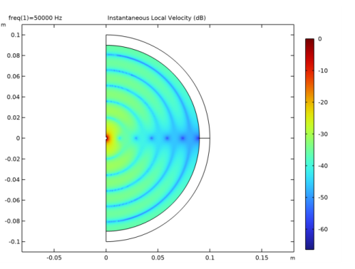
In the Settings window for 2D Plot Group, type Instantaneous Local Velocity (dB) in the Label text field.
3
Click to expand the Selection section. From the Geometric entity level list, choose Domain.
4
Click to expand the Title section. From the Title type list, choose Label.
Surface 1
1
Right-click Instantaneous Local Velocity (dB) and choose Surface.
The acoustic velocity quickly fades away as the distance from the particle grows. Use the logarithmic scale with the reference value U0 for better visualization of the velocity profile.
2
In the Settings window for Surface, locate the Expression section.
3
In the Expression text field, type 10*log10(abs(ta.v_inst/U0))[dB].
4
In the Instantaneous Local Velocity (dB) toolbar, click  Plot.
The figure should look like the one in Figure 3.
Next, create two Cut Line 2D datasets to compare the numerical thermoviscous results, the analytical (adiabatic/asymptotic), and the pressure acoustics solutions with the boundary layer impedance condition. The first spans half the air domain and the second extends 20 viscous boundary layers from the particle.
Cut Line 2D 1
1
In the Results toolbar, click  Cut Line 2D.
2
In the Settings window for Cut Line 2D, locate the Line Data section.
3
In row Point 1, set R to a_s/sqrt(2).
4
In row Point 1, set Z to a_s/sqrt(2).
5
In row Point 2, set R to 0.5*a_ta/sqrt(2).
6
In row Point 2, set Z to 0.5*a_ta/sqrt(2).
Cut Line 2D 2
1
In the Results toolbar, click  Cut Line 2D.
2
In the Settings window for Cut Line 2D, locate the Line Data section.
3
In row Point 1, set R to a_s/sqrt(2).
4
In row Point 1, set Z to a_s/sqrt(2).
5
In row Point 2, set R to (a_s+20*dvisc)/sqrt(2).
6
In row Point 2, set Z to (a_s+20*dvisc)/sqrt(2).
Acoustic Pressure vs. Distance
1
In the Results toolbar, click  1D Plot Group.
2
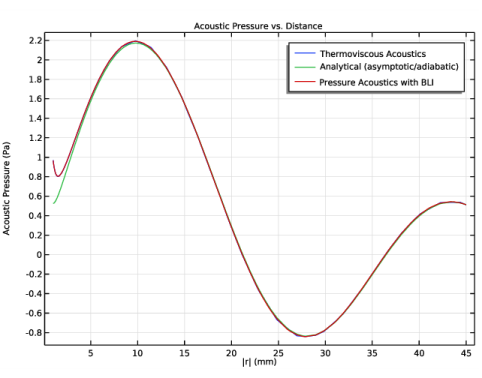
In the Settings window for 1D Plot Group, type Acoustic Pressure vs. Distance in the Label text field.
3
Locate the Data section. From the Dataset list, choose Cut Line 2D 1.
4
Click to expand the Title section. From the Title type list, choose Label.
5
Locate the Plot Settings section. Select the x-axis label check box.
6
7
Select the y-axis label check box.
8
Line Graph 1
1
Right-click Acoustic Pressure vs. Distance and choose Line Graph.
2
In the Settings window for Line Graph, locate the x-Axis Data section.
3
From the Parameter list, choose Expression.
4
In the Expression text field, type R0.
5
From the Unit list, choose mm.
6
Click to expand the Legends section. Select the Show legends check box.
7
From the Legends list, choose Manual.
8
Line Graph 2
1
Right-click Line Graph 1 and choose Duplicate.
2
In the Settings window for Line Graph, locate the y-Axis Data section.
3
In the Expression text field, type p_an.
4
Locate the Legends section. In the table, enter the following settings:
Line Graph 3
1
Right-click Line Graph 2 and choose Duplicate.
2
In the Settings window for Line Graph, locate the y-Axis Data section.
3
In the Expression text field, type acpr.p_t.
4
Locate the Legends section. In the table, enter the following settings:
5
In the Acoustic Pressure vs. Distance toolbar, click  Plot.
The figure should look like the one in Figure 4.
Axial Velocity vs. Distance
1
In the Home toolbar, click  Add Plot Group and choose 1D Plot Group.
2
In the Settings window for 1D Plot Group, type Axial Velocity vs. Distance in the Label text field.
3
Locate the Data section. From the Dataset list, choose Cut Line 2D 2.
4
Click to expand the Title section. From the Title type list, choose Label.
5
Locate the Plot Settings section. Select the x-axis label check box.
6
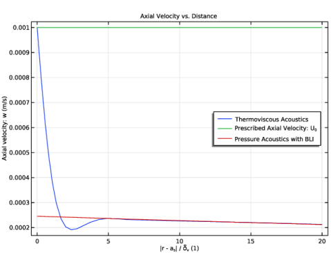
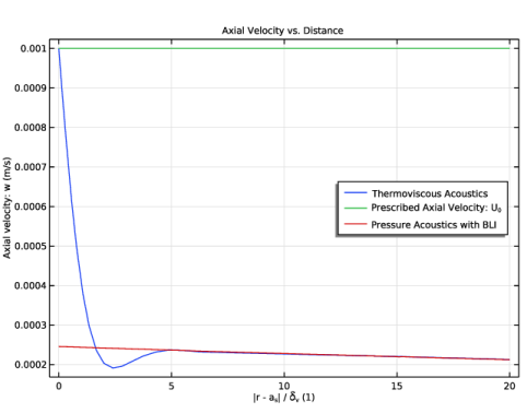
In the associated text field, type |r - a<sub>s</sub>| / \delta<sub>v</sub> (1).
7
Select the y-axis label check box.
8
In the associated text field, type Axial velocity: w (m/s).
9
Locate the Legend section. From the Position list, choose Middle right.
Line Graph 1
1
Right-click Axial Velocity vs. Distance and choose Line Graph.
2
In the Settings window for Line Graph, locate the y-Axis Data section.
3
In the Expression text field, type w.
4
Locate the x-Axis Data section. From the Parameter list, choose Expression.
5
In the Expression text field, type (R0-a_s)/dvisc.
6
Click to expand the Legends section. Select the Show legends check box.
7
From the Legends list, choose Manual.
8
Line Graph 2
1
Right-click Line Graph 1 and choose Duplicate.
2
In the Settings window for Line Graph, locate the y-Axis Data section.
3
In the Expression text field, type U0.
4
Locate the Legends section. In the table, enter the following settings:
Line Graph 3
1
Right-click Line Graph 2 and choose Duplicate.
2
In the Settings window for Line Graph, locate the y-Axis Data section.
3
In the Expression text field, type acpr.vz.
4
Locate the Legends section. In the table, enter the following settings:
5
In the Axial Velocity vs. Distance toolbar, click  Plot.
The figure should look like the one below. It shows the radial velocity close to the particle surface. Notice how the results from pressure acoustics, that use the thermoviscous boundary layer impedance (BLI) condition, match the full thermovsicous model except in the boundary layer itself. The BLI condition treats what happens in the layer analytically.