|
|
|

|
1
|
|
2
|
In the Select Physics tree, select Acoustics>Pressure Acoustics>Pressure Acoustics, Frequency Domain (acpr).
|
|
3
|
Click Add.
|
|
4
|
|
5
|
Click Add.
|
|
6
|
Click
|
|
7
|
|
8
|
Click
|
|
1
|
|
2
|
|
1
|
|
2
|
|
3
|
|
4
|
|
5
|
|
1
|
|
2
|
|
3
|
|
1
|
|
2
|
|
3
|
|
4
|
|
5
|
|
1
|
|
2
|
|
3
|
|
4
|
|
5
|
|
1
|
|
2
|
Click in the Graphics window and then press Ctrl+A to select both objects.
|
|
3
|
|
1
|
|
2
|
|
3
|
|
4
|
|
5
|
|
6
|
Click to expand the Layers section. In the table, enter the following settings:
|
|
7
|
|
8
|
|
9
|
|
10
|
|
1
|
|
2
|
|
3
|
|
4
|
|
5
|
|
6
|
Locate the Layers section. In the table, enter the following settings:
|
|
7
|
|
8
|
|
9
|
|
1
|
|
2
|
|
3
|
|
4
|
|
5
|
|
6
|
|
7
|
Click to expand the Layers section. In the table, enter the following settings:
|
|
8
|
|
1
|
|
2
|
|
3
|
|
1
|
|
2
|
|
3
|
|
1
|
|
2
|
|
3
|
|
4
|
|
5
|
|
6
|
|
7
|
|
8
|
|
1
|
|
2
|
|
1
|
|
2
|
|
4
|
|
5
|
|
6
|
|
1
|
|
3
|
|
4
|
|
5
|
|
1
|
In the Model Builder window, under Component 1 (comp1) click Pressure Acoustics, Frequency Domain (acpr).
|
|
2
|
In the Settings window for Pressure Acoustics, Frequency Domain, locate the Sound Pressure Level Settings section.
|
|
3
|
From the Reference pressure for the sound pressure level list, choose Use reference pressure for water.
|
|
4
|
Locate the Typical Wave Speed for Perfectly Matched Layers section. In the cref text field, type 1483[m/s].
|
|
1
|
In the Model Builder window, under Component 1 (comp1)>Pressure Acoustics, Frequency Domain (acpr) click Pressure Acoustics 1.
|
|
2
|
|
3
|
|
4
|
|
1
|
|
3
|
|
4
|
|
5
|
|
1
|
|
3
|
|
4
|
|
1
|
|
2
|
|
3
|
|
1
|
In the Model Builder window, under Component 1 (comp1)>Bioheat Transfer (ht) click Initial Values 1.
|
|
2
|
|
3
|
|
1
|
|
3
|
|
4
|
|
1
|
|
3
|
|
4
|
|
1
|
|
2
|
|
3
|
|
4
|
|
5
|
|
1
|
In the Model Builder window, under Component 1 (comp1) right-click Materials and choose Blank Material.
|
|
2
|
|
4
|
|
1
|
In the Model Builder window, under Component 1 (comp1)>Pressure Acoustics, Frequency Domain (acpr) click Pressure Acoustics 1.
|
|
2
|
|
3
|
|
1
|
|
2
|
|
3
|
|
1
|
|
2
|
|
1
|
|
2
|
|
3
|
|
1
|
|
2
|
|
3
|
|
5
|
|
6
|
|
7
|
In the associated text field, type 1568[m/s]/f0/30.
|
|
1
|
|
2
|
|
3
|
Click the Custom button.
|
|
4
|
Locate the Element Size Parameters section. In the Maximum element size text field, type 1483[m/s]/f0/5.
|
|
1
|
|
2
|
|
3
|
|
1
|
|
3
|
|
4
|
|
5
|
|
1
|
|
2
|
|
1
|
|
2
|
|
3
|
|
1
|
|
3
|
|
4
|
Click the Custom button.
|
|
5
|
|
6
|
In the associated text field, type 0.18[mm].
|
|
1
|
|
2
|
|
3
|
Click the Custom button.
|
|
4
|
|
5
|
|
6
|
|
1
|
|
2
|
|
3
|
|
4
|
Locate the Physics and Variables Selection section. In the table, clear the Solve for check box for Bioheat Transfer (ht).
|
|
5
|
|
6
|
|
7
|
|
8
|
|
1
|
|
2
|
|
3
|
Find the Studies subsection. In the Select Study tree, select Preset Studies for Some Physics Interfaces>Time Dependent.
|
|
4
|
Find the Physics interfaces in study subsection. In the table, clear the Solve check box for Pressure Acoustics, Frequency Domain (acpr).
|
|
5
|
|
6
|
|
1
|
|
2
|
Click
|
|
3
|
|
4
|
|
5
|
Click Replace.
|
|
6
|
In the Settings window for Time Dependent, click to expand the Values of Dependent Variables section.
|
|
7
|
Find the Values of variables not solved for subsection. From the Settings list, choose User controlled.
|
|
8
|
|
9
|
|
10
|
|
11
|
|
12
|
|
1
|
|
2
|
|
3
|
|
4
|
|
5
|
|
6
|
|
7
|
|
1
|
|
2
|
|
3
|
|
4
|
|
5
|
In the associated text field, type r coordinate (mm).
|
|
6
|
|
7
|
In the associated text field, type z coordinate (mm).
|
|
8
|
|
1
|
|
2
|
|
3
|
|
1
|
|
2
|
|
3
|
|
4
|
Click in the Graphics window and then press Ctrl+A to select all domains.
|
|
1
|
|
2
|
|
3
|
|
4
|
|
5
|
In the associated text field, type r coordinate (mm).
|
|
6
|
|
7
|
In the associated text field, type z coordinate (mm).
|
|
8
|
|
1
|
|
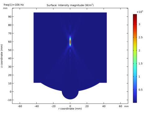
2
|
In the Settings window for Surface, click Replace Expression in the upper-right corner of the Expression section. From the menu, choose Component 1 (comp1)>Pressure Acoustics, Frequency Domain>Intensity>acpr.I_mag - Intensity magnitude - W/m².
|
|
3
|
|
1
|
|
2
|
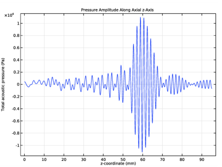
In the Settings window for 1D Plot Group, type Pressure Amplitude Along Axial z-Axis in the Label text field.
|
|
3
|
|
1
|
|
3
|
|
4
|
|
5
|
|
6
|
|
1
|
|
2
|
|
3
|
|
4
|
|
5
|
Click
|
|
1
|
|
2
|
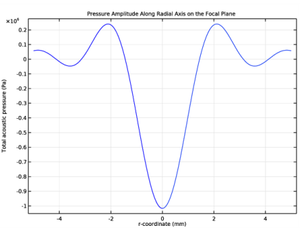
In the Settings window for 1D Plot Group, type Pressure Amplitude Along Radial Axis on the Focal Plane in the Label text field.
|
|
3
|
|
4
|
|
5
|
|
6
|
In the associated text field, type r-coordinate (mm).
|
|
1
|
|
2
|
|
3
|
|
4
|
|
5
|
|
6
|
|
1
|
|
2
|
|
3
|
|
4
|
|
5
|
|
1
|
|
2
|
|
3
|
|
1
|
|
2
|
|
3
|
|
4
|
|
5
|
|
6
|
|
7
|
|
8
|
In the associated text field, type r coordinate (mm).
|
|
9
|
|
10
|
In the associated text field, type z coordinate (mm).
|
|
11
|
|
1
|
|
2
|
|
3
|
|
4
|
|
5
|
|
6
|
|
1
|
|
2
|
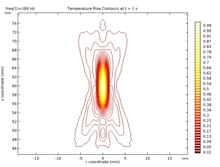
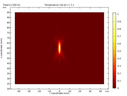
In the Settings window for 2D Plot Group, type Isothermal Contours at t = 1 s in the Label text field.
|
|
3
|
|
4
|
|
5
|
|
6
|
|
7
|
|
8
|
In the associated text field, type r coordinate (mm).
|
|
9
|
|
10
|
In the associated text field, type z coordinate (mm).
|
|
11
|
|
1
|
|
2
|
|
3
|
|
4
|
|
5
|
|
6
|
|
7
|
|
1
|
|
2
|
|
3
|
|
4
|
|
5
|
|
1
|
|
2
|
|
3
|
|
1
|
|
2
|
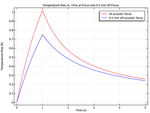
In the Settings window for 1D Plot Group, type Temperature Rise vs. Time at Focus and 0.5 mm off Focus in the Label text field.
|
|
3
|
Locate the Data section. From the Dataset list, choose Study 2 - Bioheat Transfer/Solution 2 (sol2).
|
|
4
|
|
5
|
|
6
|
In the associated text field, type Temperature Rise (K).
|
|
1
|
|
2
|
|
3
|
|
4
|
|
5
|
|
6
|
|
7
|
|
8
|
|
1
|
|
2
|
|
3
|
|
4
|
|
5
|
|
6
|
Locate the Legends section. In the table, enter the following settings:
|
|
7
|
|
8
|
|
1
|
|
2
|
|
3
|
|
1
|
|
2
|
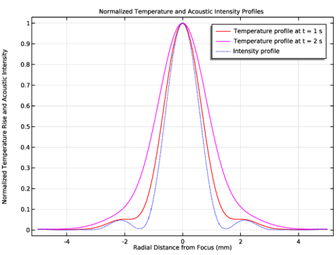
In the Settings window for 1D Plot Group, type Normalized Temperature and Acoustic Intensity Profiles in the Label text field.
|
|
3
|
|
4
|
|
5
|
In the associated text field, type Radial Distance from Focus (mm).
|
|
6
|
|
7
|
In the associated text field, type Normalized Temperature Rise and Acoustic Intensity.
|
|
1
|
|
2
|
|
3
|
|
4
|
|
5
|
|
6
|
|
7
|
|
8
|
|
9
|
|
10
|
|
11
|
|
1
|
|
2
|
|
3
|
|
4
|
|
1
|
In the Model Builder window, under Results>Normalized Temperature and Acoustic Intensity Profiles right-click Line Graph 1 and choose Duplicate.
|
|
2
|
|
3
|
|
4
|
|
5
|
|
6
|
Locate the Legends section. In the table, enter the following settings:
|
|
1
|
|
2
|
|
3
|
|
4
|
|
1
|
In the Model Builder window, under Results>Normalized Temperature and Acoustic Intensity Profiles right-click Line Graph 1 and choose Duplicate.
|
|
2
|
|
3
|
|
4
|
Click Replace Expression in the upper-right corner of the y-Axis Data section. From the menu, choose Component 1 (comp1)>Pressure Acoustics, Frequency Domain>Intensity>acpr.I_mag - Intensity magnitude - W/m².
|
|
5
|
|
6
|
|
7
|
|
8
|
Locate the Legends section. In the table, enter the following settings:
|
|
1
|
|
2
|
|
3
|
|
4
|
|
5
|