|
|
|

|
1.18·10-3 m/N
|
||
|
7 Ω
|
||
|
|
||
|
|
||
|
|
||
|
|
||
|
|
||
|
|
||
 |


|
1
|
|
2
|
In the Select Physics tree, select Acoustics>Pressure Acoustics>Pressure Acoustics, Frequency Domain (acpr).
|
|
3
|
Click Add.
|
|
4
|
|
5
|
Click Add.
|
|
6
|
Click
|
|
7
|
|
8
|
Click
|
|
1
|
|
2
|
|
3
|
|
4
|
Browse to the model’s Application Libraries folder and double-click the file lumped_loudspeaker_driver_parameters.txt.
|
|
1
|
|
2
|
|
3
|
|
4
|
|
5
|
|
1
|
|
2
|
|
3
|
|
4
|
|
5
|
|
6
|
Click to expand the Layers section. In the table, enter the following settings:
|
|
1
|
|
2
|
|
3
|
|
4
|
Locate the Coordinates section. In the table, enter the following settings:
|
|
1
|
|
2
|
|
3
|
|
4
|
Locate the Coordinates section. In the table, enter the following settings:
|
|
5
|
|
6
|
|
1
|
|
2
|
|
3
|
|
4
|
|
5
|
|
6
|
|
7
|
|
8
|
|
9
|
|
1
|
|
2
|
On the object c1, select Boundaries 3 and 4 only.
|
|
3
|
|
1
|
|
2
|
|
3
|
|
4
|
Locate the Coordinates section. In the table, enter the following settings:
|
|
5
|
|
1
|
|
2
|
|
3
|
|
4
|
Browse to the model’s Application Libraries folder and double-click the file lumped_loudspeaker_driver_variables_1.txt.
|
|
1
|
|
2
|
|
3
|
|
4
|
Browse to the model’s Application Libraries folder and double-click the file lumped_loudspeaker_driver_variables_2.txt.
|
|
1
|
|
2
|
|
3
|
|
1
|
|
2
|
|
3
|
|
1
|
|
2
|
|
3
|
|
1
|
|
3
|
|
4
|
|
5
|
|
6
|
|
1
|
|
2
|
|
3
|
In the tree, select Built-in>Air.
|
|
4
|
|
5
|
|
1
|
In the Model Builder window, under Component 1 (comp1) right-click Pressure Acoustics, Frequency Domain (acpr) and choose Interior Conditions>Interior Sound Hard Boundary (Wall).
|
|
2
|
In the Settings window for Interior Sound Hard Boundary (Wall), locate the Boundary Selection section.
|
|
3
|
|
1
|
|
2
|
|
3
|
|
1
|
|
3
|
In the Settings window for Exterior Field Calculation, locate the Exterior Field Calculation section.
|
|
4
|
|
1
|
|
2
|
In the Settings window for Interior Sound Hard Boundary (Wall), locate the Boundary Selection section.
|
|
3
|
|
1
|
|
2
|
|
4
|
|
1
|
|
2
|
|
4
|
|
1
|
|
2
|
|
4
|
|
1
|
|
2
|
|
4
|
|
1
|
|
2
|
|
4
|
|
1
|
|
2
|
|
4
|
|
1
|
|
2
|
|
4
|
|
5
|
Locate the Current Measurement section. From the Measure current for device list, choose Resistor 2 (R2).
|
|
1
|
|
2
|
|
4
|
|
1
|
|
2
|
In the Settings window for Current-Controlled Voltage Source, locate the Current Measurement section.
|
|
3
|
|
1
|
|
2
|
|
4
|
|
1
|
|
2
|
|
4
|
|
1
|
|
2
|
|
4
|
Locate the External Device section. From the V list, choose Voltage from lumped speaker boundary (acpr/ilsb1).
|
|
1
|
|
2
|
|
3
|
|
1
|
|
2
|
|
1
|
|
2
|
|
3
|
Click
|
|
4
|
|
5
|
|
6
|
|
7
|
|
8
|
Click Replace.
|
|
9
|
|
10
|
|
11
|
In the tree, select Component 1 (Comp1)>Pressure Acoustics, Frequency Domain (Acpr)>Interior Sound Hard Boundary (Wall) 2.
|
|
12
|
Click
|
|
13
|
|
14
|
|
15
|
|
16
|
|
17
|
|
18
|
|
1
|
|
2
|
|
3
|
|
1
|
|
2
|
|
3
|
|
4
|
|
5
|
|
6
|
|
7
|
|
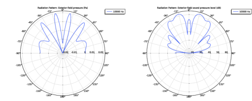
1
|
In the Model Builder window, expand the Exterior-Field Sound Pressure Level (acpr) node, then click Radiation Pattern 1.
|
|
2
|
|
3
|
|
4
|
|
5
|
|
6
|
|
1
|
In the Model Builder window, expand the Exterior-Field Pressure (acpr) node, then click Radiation Pattern 1.
|
|
2
|
|
3
|
|
4
|
|
5
|
|
6
|
|
8
|
|
1
|
|
2
|
|
3
|
|
4
|
|
5
|
|
6
|
|
7
|
In the associated text field, type Velocity amplitude (m/s).
|
|
1
|
|
2
|
|
4
|
|
5
|
|
1
|
|
2
|
|
3
|
|
4
|
|
5
|
|
6
|
|
7
|
In the associated text field, type Power (W).
|
|
8
|
|
1
|
|
2
|
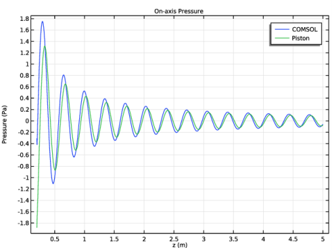
In the Settings window for Global, click Add Expression in the upper-right corner of the y-Axis Data section. From the menu, choose Component 1 (comp1)>Definitions>Variables>P_AR - Radiated power (COMSOL) - W.
|
|
3
|
Click Add Expression in the upper-right corner of the y-Axis Data section. From the menu, choose Component 1 (comp1)>Definitions>Variables>P_AR_ana - Radiated power (piston) - W.
|
|
4
|
|
5
|
|
1
|
|
2
|
|
3
|
|
4
|
|
5
|
|
6
|
|
7
|
In the associated text field, type Power (W).
|
|
8
|
|
1
|
|
2
|
In the Settings window for Global, click Replace Expression in the upper-right corner of the y-Axis Data section. From the menu, choose Component 1 (comp1)>Definitions>Variables>P_E - Electric input power (rms) - W.
|
|
3
|
|
4
|
|
1
|
|
2
|
|
3
|
|
4
|
|
5
|
|
6
|
|
7
|
In the associated text field, type Efficiency (%).
|
|
8
|
|
1
|
|
2
|
|
4
|
|
5
|
|
1
|
|
2
|
|
3
|
|
4
|
|
5
|
|
6
|
|
7
|
In the associated text field, type Pressure force (N).
|
|
8
|
|
1
|
|
2
|
|
4
|
|
5
|
|
1
|
|
2
|
|
3
|
|
4
|
|
5
|
|
6
|
|
7
|
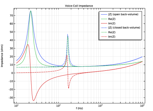
In the associated text field, type Impedance (ohm).
|
|
1
|
|
2
|
|
4
|
|
5
|
|
1
|
|
2
|
|
3
|
|
4
|
|
5
|
|
6
|
|
7
|
In the associated text field, type Level (dB SPL rel. 1 V).
|
|
8
|
|
1
|
|
2
|
|
3
|
|
4
|
|
5
|
|
6
|
|
7
|
|
9
|
|
1
|
|
2
|
|
3
|
|
4
|
Locate the Legends section. In the table, enter the following settings:
|
|
5
|
|
1
|
|
2
|
In the Settings window for 1D Plot Group, type Phase Relative to a Plane Wave in the Label text field.
|
|
3
|
|
4
|
|
5
|
|
6
|
|
7
|
In the associated text field, type Phase (deg).
|
|
8
|
|
1
|
|
2
|
|
4
|
|
5
|
|
1
|
|
2
|
|
3
|
|
4
|
|
1
|
|
2
|
|
3
|
|
4
|
|
5
|
|
6
|
|
7
|
|
8
|
In the associated text field, type Pressure (Pa).
|
|
9
|
|
10
|
|
1
|
|
2
|
|
3
|
|
4
|
|
5
|
|
6
|
|
7
|
|
8
|
|
1
|
|
2
|
|
3
|
|
4
|
Locate the Legends section. In the table, enter the following settings:
|
|
5
|
|
1
|
|
2
|
|
1
|
|
2
|
|
3
|
|
1
|
|
2
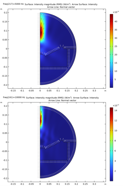
|
In the Settings window for Arrow Surface, click Replace Expression in the upper-right corner of the Expression section. From the menu, choose Component 1 (comp1)>Pressure Acoustics, Frequency Domain>Intensity>acpr.Ir,acpr.Iz - Intensity.
|
|
3
|
|
1
|
|
2
|
In the Settings window for Arrow Line, click Replace Expression in the upper-right corner of the Expression section. From the menu, choose Component 1 (comp1)>Pressure Acoustics, Frequency Domain>Geometry>acpr.nr,acpr.nz - Normal vector.
|
|
3
|
|
4
|
|
5
|
|
1
|
|
2
|
|
3
|
|
4
|
|
5
|
|
6
|
|
7
|
|
8
|
|
1
|
|
2
|
|
1
|
|
2
|
|
3
|
|
4
|
|
5
|
|
6
|
|
7
|
|
8
|
|
9
|
|
1
|
|
2
|
|
3
|
|
1
|
|
2
|
|
1
|
|
2
|
|
3
|
|
4
|
|
1
|
|
2
|
|
3
|
|
4
|
|
1
|
|
2
|
|
3
|
|
4
|
|
5
|
|
6
|
|
7
|
|
8
|
|
9
|
|
10
|
|
11
|
In the associated text field, type Phase (deg).
|
|
12
|
|
1
|
|
2
|
|
3
|
|
4
|
|
5
|
|
1
|
|
2
|
Click
|
|
3
|
|
4
|
|
5
|
|
6
|
|
7
|
Click Replace.
|
|
8
|
|
9
|
|
10
|
|
11
|
|
1
|
|
2
|
|
1
|
|
2
|
|
3
|
|
4
|
|
5
|
|
6
|
|
7
|
|
1
|
|
2
|
|
1
|
|
2
|
|
3
|
|
4
|
Locate the Legends section. In the table, enter the following settings:
|
|
5
|