PDF

Jet Pipe
Introduction
This example models the radiation of fan noise from the annular duct of a turbofan aeroengine. When the jet stream excites the duct, a vortex sheet appears along the extension of the duct wall. In the model you calculate the near field on both sides of the vortex sheet. The background mean-flow is assumed to be well described by a potential flow, in this model a uniform flow. This means that, the acoustic field can be modeled by solving the linearized potentiality flow equations in the frequency domain.
Model Definition
The model is axisymmetric with the symmetry axis coinciding with the engine’s centerline (gray area in the figure below). The flows both inside and outside the duct are uniform mean flows, they have a magnitude of M1 and M0, respectively. Because the flow velocities differ, a vortex sheet separates them (dashed line in the figure below).
Sketch of the turbofan motor.
The Linearized Potential Flow, Frequency Domain interface in the Acoustics Module describes acoustic waves in a moving fluid with the potential φ, for the local particle velocity as the basic dependent variable; see the chapter about aeroacoustics in the Acoustics Module User’s Guide for details. The field equations are only valid when the background velocity field is irrotational, a condition that is not satisfied across a vortex sheet. As a consequence, the velocity potential is discontinuous across this sheet. To model this discontinuity, you use the Vortex Sheet boundary condition which is available on interior boundaries. The boundary conditions on the two sides of the vortex sheet are defined as follows:
In these equations, ω is the angular velocity, V is the mean-flow velocity, w is the outward normal displacement, φ is the velocity potential, and p is the pressure. The subscripts “up” and “down” refer to the two sides of the boundary.
The velocity normal to the vortex sheet is zero, which implies that the last two terms on the left-hand side of the condition vanishes. In the model the variables are made dimensionless. The velocities are divided by the speed of sound in air and the densities are divided by the density for air. For example, the model uses the Mach number M = V/c0 as the mean flow velocity. This leads to the boundary conditions
where M denotes the transverse Mach number.
The duct has a hard wall, which you also model using an interior boundary condition.
The acoustic field inside the duct can be described as a sum of eigenmodes propagating in the duct and then radiating in the free space. This is discussed in section 2.1 in Ref. 1. In this example you study the radiated acoustic waves produced by a single eigenmode at a time. First you calculate the eigenmodes with the azimuthal mode number 4 on the inlet boundary. From these eigenmodes, the one with radial mode order 0 is used as incident wave. You then calculate the velocity fields with azimuthal mode numbers m = 17 and 24 and with radial mode order n = 1.
Results and Discussion
The inlet sources are found using a boundary mode analysis. The analysis is made with the circumferential wave number m = 4, 17, and 24 and gives several eigenmodes corresponding to different radial mode numbers. This example, like Ref. 1, uses the eigenmodes (m,n) = (4,0), (17,1), and (24,1) as incident waves in the duct. The modes are depicted in Figure 1. The radial mode n = 0 corresponds to the largest eigenvalue for a given m, while n = 1 corresponds to the smallest eigenvalue.
Figure 1: Mode shape for m = 4, 17, and 24 for both n = 0 and n=1
In Figure 2 the source velocity potential is depicted in the revolved geometry including the azimuthal mode contribution, given as
where m is the mode number and is the azimuthal angle.
The near field pressure around the duct obtained by COMSOL Multiphysics can be compared to the results for the near field in Ref. 1. Figure 3 through Figure 7 show the near-field solution for a Mach number equal to M1 = 0.45 in the pipe and M0 = 0.25 on the outside. The figures show the pressure field for the different source eigenmodes shown in Figure 1.
Figure 2: The boundary mode (m,n) = (4,0) depicted in the revolved geometry including the azimuthal wave number contribution.
Figure 3: The near-field solution for m = 4 and n = 0.
Figure 4: The near-field solution for m = 17 and n = 1.
Figure 5: The near-field solution for m = 24 and n = 1.
Figure 6: The near-field sound pressure level for m = 24 and n = 1.
Figure 7: The near-field pressure plotted in the revolved geometry for m = 4 and n = 0.
Reference
1. G. Gabard and R.J. Astley, “Theoretical Model for Sound Radiations from Annular Jet Pipes: Far- and Near-field Solution,” J. Fluid Mech., vol. 549, pp. 315–341, 2006.
Application Library path: Acoustics_Module/Aeroacoustics_and_Noise/jet_pipe
Modeling Instructions
From the File menu, choose New.
New
In the New window, click  Model Wizard.
Model Wizard
1
In the Model Wizard window, click  2D Axisymmetric.
2
In the Select Physics tree, select Acoustics>Aeroacoustics>Linearized Potential Flow, Boundary Mode (aebm).
3
Click Add.
4
In the Select Physics tree, select Acoustics>Aeroacoustics>Linearized Potential Flow, Frequency Domain (ae).
5
Click Add.
6
Click  Study.
7
In the Select Study tree, select Preset Studies for Some Physics Interfaces>Mode Analysis.
8
Root
1
In the Model Builder window, click the root node.
2
In the root node’s Settings window, locate the Unit System section.
3
From the Unit system list, choose None.
This setting turns off all unit support in the model.
Geometry 1
Rectangle 1 (r1)
1
In the Geometry toolbar, click  Rectangle.
2
In the Settings window for Rectangle, locate the Size and Shape section.
3
In the Width text field, type 0.25.
4
In the Height text field, type 0.5.
5
Locate the Position section. In the r text field, type 0.75.
6
In the z text field, type -0.5.
Rectangle 2 (r2)
1
In the Geometry toolbar, click  Rectangle.
2
In the Settings window for Rectangle, locate the Size and Shape section.
3
In the Width text field, type 0.25.
4
Locate the Position section. In the r text field, type 0.75.
Rectangle 3 (r3)
1
In the Geometry toolbar, click  Rectangle.
2
In the Settings window for Rectangle, locate the Size and Shape section.
3
In the Width text field, type 0.25.
4
In the Height text field, type 0.2.
5
Locate the Position section. In the r text field, type 0.75.
6
In the z text field, type 1.
7
Click the  Zoom Extents button in the Graphics toolbar.
Rectangle 4 (r4)
1
In the Geometry toolbar, click  Rectangle.
2
In the Settings window for Rectangle, locate the Size and Shape section.
3
In the Height text field, type 1.5.
4
Locate the Position section. In the r text field, type 1.
5
In the z text field, type -0.5.
6
Click the  Zoom Extents button in the Graphics toolbar.
Rectangle 5 (r5)
1
In the Geometry toolbar, click  Rectangle.
2
In the Settings window for Rectangle, locate the Size and Shape section.
3
In the Width text field, type 1.2.
4
In the Height text field, type 0.2.
5
Locate the Position section. In the r text field, type 1.
6
In the z text field, type -0.7.
Rectangle 6 (r6)
1
In the Geometry toolbar, click  Rectangle.
2
In the Settings window for Rectangle, locate the Size and Shape section.
3
In the Width text field, type 0.2.
4
In the Height text field, type 1.9.
5
Locate the Position section. In the r text field, type 2.
6
In the z text field, type -0.7.
Rectangle 7 (r7)
1
In the Geometry toolbar, click  Rectangle.
2
In the Settings window for Rectangle, locate the Size and Shape section.
3
In the Width text field, type 1.2.
4
In the Height text field, type 0.2.
5
Locate the Position section. In the r text field, type 1.
6
In the z text field, type 1.
7
Click  Build All Objects.
8
Click the  Zoom Extents button in the Graphics toolbar.
This completes the geometry-modeling state. The geometry in the Graphics window should now look like that in the figure below.
Global Definitions
Parameters 1
1
In the Model Builder window, under Global Definitions click Parameters 1.
2
In the Settings window for Parameters, locate the Parameters section.
3
Definitions
Duct Cross Section
1
In the Definitions toolbar, click  Explicit.
2
In the Settings window for Explicit, type Duct Cross Section in the Label text field.
3
Locate the Input Entities section. From the Geometric entity level list, choose Boundary.
4
Materials
Specify the density and speed of sound, both normalized to 1, as material parameters. You need to add a separate material node for the duct cross section because it is a boundary and not a domain.
Material 1 (mat1)
1
In the Model Builder window, under Component 1 (comp1) right-click Materials and choose Blank Material.
2
In the Settings window for Material, locate the Material Contents section.
3
Material 2 (mat2)
1
Right-click Materials and choose Blank Material.
2
In the Settings window for Material, locate the Geometric Entity Selection section.
3
From the Geometric entity level list, choose Boundary.
4
From the Selection list, choose Duct Cross Section.
5
Locate the Material Contents section. In the table, enter the following settings:
Linearized Potential Flow, Boundary Mode (aebm)
1
In the Model Builder window, under Component 1 (comp1) click Linearized Potential Flow, Boundary Mode (aebm).
2
In the Settings window for Linearized Potential Flow, Boundary Mode, locate the Boundary Selection section.
3
From the Selection list, choose Duct Cross Section.
4
Click to expand the Equation section. Locate the Linearized Potential Flow Equation Settings section. In the m text field, type m.
Linearized Potential Flow Model 1
1
In the Model Builder window, under Component 1 (comp1)>Linearized Potential Flow, Boundary Mode (aebm) click Linearized Potential Flow Model 1.
2
In the Settings window for Linearized Potential Flow Model, locate the Linearized Potential Flow Model section.
3
Specify the V vector as
Linearized Potential Flow, Frequency Domain (ae)
1
In the Model Builder window, under Component 1 (comp1) click Linearized Potential Flow, Frequency Domain (ae).
2
In the Settings window for Linearized Potential Flow, Frequency Domain, locate the Linearized Potential Flow Equation Settings section.
3
In the m text field, type m.
4
Locate the Typical Wave Speed for Perfectly Matched Layers section. In the cref text field, type 1[m/s].
Linearized Potential Flow Model 1
1
In the Model Builder window, under Component 1 (comp1)>Linearized Potential Flow, Frequency Domain (ae) click Linearized Potential Flow Model 1.
2
In the Settings window for Linearized Potential Flow Model, locate the Linearized Potential Flow Model section.
3
Specify the V vector as
Vortex Sheet 1
1
In the Physics toolbar, click  Boundaries and choose Vortex Sheet.
2
Interior Sound Hard Boundary (Wall) 1
1
In the Physics toolbar, click  Boundaries and choose Interior Sound Hard Boundary (Wall).
2
Linearized Potential Flow Model 2
1
In the Physics toolbar, click  Domains and choose Linearized Potential Flow Model.
2
3
In the Settings window for Linearized Potential Flow Model, locate the Linearized Potential Flow Model section.
4
Specify the V vector as
Velocity Potential 1
1
In the Physics toolbar, click  Boundaries and choose Velocity Potential.
The value of the velocity potential is given by the boundary mode solutions. The dependent variable is phi.
2
In the Settings window for Velocity Potential, locate the Boundary Selection section.
3
From the Selection list, choose Duct Cross Section.
4
Locate the Velocity Potential section. In the φ0 text field, type phi.
Definitions
Perfectly Matched Layer 1 (pml1)
1
In the Definitions toolbar, click  Perfectly Matched Layer.
2
3
In the Settings window for Perfectly Matched Layer, locate the Geometry section.
4
From the Type list, choose Cylindrical.
5
Locate the Scaling section. From the Coordinate stretching type list, choose Rational.
In this model, the mesh is set up manually. Proceed by directly adding the desired mesh component.
Mesh 1
Free Triangular 1
1
In the Mesh toolbar, click  Free Triangular.
2
In the Settings window for Free Triangular, locate the Domain Selection section.
3
From the Geometric entity level list, choose Domain.
4
Size
1
In the Model Builder window, click Size.
2
In the Settings window for Size, locate the Element Size section.
3
Click the Custom button.
4
Locate the Element Size Parameters section. In the Maximum element size text field, type (1-M1)/f/6.
5
In the Minimum element size text field, type (1-M1)/f/6.
Mapped 1
In the Mesh toolbar, click  Mapped.
Distribution 1
1
Right-click Mapped 1 and choose Distribution.
2
3
In the Settings window for Distribution, locate the Distribution section.
4
In the Number of elements text field, type 8.
5
Click  Build All.
Start by solving the boundary mode problem to find the source potentials that will be applied in the full model.
Study 1 - Mode Analysis
1
In the Model Builder window, click Study 1.
2
In the Settings window for Study, type Study 1 - Mode Analysis in the Label text field.
3
Locate the Study Settings section. Clear the Generate default plots check box.
Parametric Sweep
1
In the Study toolbar, click  Parametric Sweep.
2
In the Settings window for Parametric Sweep, locate the Study Settings section.
3
4
Step 1: Mode Analysis
1
In the Model Builder window, click Step 1: Mode Analysis.
2
In the Settings window for Mode Analysis, locate the Study Settings section.
3
In the Mode analysis frequency text field, type f.
4
From the Mode search method around shift list, choose Smaller real part.
5
Select the Desired number of modes check box.
6
7
Select the Search for modes around check box.
8
9
Locate the Physics and Variables Selection section. In the table, clear the Solve for check box for Linearized Potential Flow, Frequency Domain (ae).
10
In the Study toolbar, click  Compute.
Results
Boundary Modes
1
In the Model Builder window, expand the Results node.
2
Right-click Results and choose 1D Plot Group.
3
In the Settings window for 1D Plot Group, type Boundary Modes in the Label text field.
4
Locate the Data section. From the Dataset list, choose Study 1 - Mode Analysis/Parametric Solutions 1 (sol2).
5
Locate the Legend section. From the Position list, choose Lower left.
Line Graph 1
1
Right-click Boundary Modes and choose Line Graph.
2
3
In the Boundary Modes toolbar, click  Plot.
4
In the Settings window for Line Graph, locate the x-Axis Data section.
5
From the Parameter list, choose Expression.
6
In the Expression text field, type r.
7
Click to expand the Legends section. Select the Show legends check box.
8
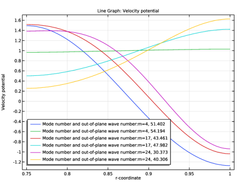
Find the Prefix and suffix subsection. In the Prefix text field, type Mode number and out-of-plane wave number: .
9
In the Boundary Modes toolbar, click  Plot.
The graph that appears should be the same as that in Figure 1. This shows the two radial modes (n=0 and 1) for m=4, 17, and 24.
Revolution 2D 1
1
In the Model Builder window, expand the Results>Datasets node.
2
Right-click Results>Datasets and choose Revolution 2D.
3
In the Settings window for Revolution 2D, locate the Data section.
4
From the Dataset list, choose Study 1 - Mode Analysis/Parametric Solutions 1 (sol2).
5
Click to expand the Advanced section. In the Azimuthal mode number text field, type m.
Boundary Modes 2D Revolved
1
In the Results toolbar, click  3D Plot Group.
2
In the Settings window for 3D Plot Group, type Boundary Modes 2D Revolved in the Label text field.
3
Locate the Data section. From the Parameter value (m) list, choose 4.
Surface 1
1
Right-click Boundary Modes 2D Revolved and choose Surface.
The circumferential behavior is automatically represented as you defined the Azimuthal mode number in the revolved solution dataset.
2
In the Boundary Modes 2D Revolved toolbar, click  Plot.
3
Click the  Zoom Extents button in the Graphics toolbar.
The graph that appears should be the same as that in Figure 2.
Now, add three studies to solve three cases with different sources: (m=4,n=0), (m=17,n=1), and (m=24,n=1), respectively. After setting up three studies and solving then plot the results.
First, solve the case with the circumferential wave number m=4 and the first radial mode (n=0), that is the mode with the highest eigenvalue.
Add Study
1
In the Home toolbar, click  Add Study to open the Add Study window.
2
Go to the Add Study window.
3
Find the Physics interfaces in study subsection. In the table, clear the Solve check box for Linearized Potential Flow, Boundary Mode (aebm).
4
Find the Studies subsection. In the Select Study tree, select General Studies>Frequency Domain.
5
Click Add Study in the window toolbar.
6
In the Home toolbar, click  Add Study to close the Add Study window.
Study 2 - m=4 and n=0
1
In the Model Builder window, click Study 2.
2
In the Settings window for Study, type Study 2 - m=4 and n=0 in the Label text field.
3
Locate the Study Settings section. Clear the Generate default plots check box.
Step 1: Frequency Domain
1
In the Model Builder window, under Study 2 - m=4 and n=0 click Step 1: Frequency Domain.
2
In the Settings window for Frequency Domain, locate the Study Settings section.
3
In the Frequencies text field, type f.
4
Click to expand the Values of Dependent Variables section. Find the Values of variables not solved for subsection. From the Settings list, choose User controlled.
5
From the Method list, choose Solution.
6
From the Study list, choose Study 1 - Mode Analysis, Mode Analysis.
7
From the Solution list, choose Parametric Solutions 1 (sol2).
8
From the Use list, choose m=4 (sol3).
9
From the Out-of-plane wave number list, choose 54.194.
The value of m is not stored in the mode analysis dataset so you need to set it manually as follows.
10
Click to expand the Study Extensions section. Select the Auxiliary sweep check box.
11
12
13
In the Home toolbar, click  Compute.
Secondly, solve the case with the circumferential wave number m=17 and the second radial mode (n=1). That is the mode with the second highest eigenvalue. The steps are the same as for Study 2.
Add Study
1
In the Home toolbar, click  Add Study to open the Add Study window.
2
Go to the Add Study window.
3
Find the Physics interfaces in study subsection. In the table, clear the Solve check box for Linearized Potential Flow, Boundary Mode (aebm).
4
Find the Studies subsection. In the Select Study tree, select General Studies>Frequency Domain.
5
Click Add Study in the window toolbar.
6
In the Home toolbar, click  Add Study to close the Add Study window.
Study 3 - m=17 and n=1
1
In the Model Builder window, click Study 3.
2
In the Settings window for Study, type Study 3 - m=17 and n=1 in the Label text field.
3
Locate the Study Settings section. Clear the Generate default plots check box.
Step 1: Frequency Domain
1
In the Model Builder window, under Study 3 - m=17 and n=1 click Step 1: Frequency Domain.
2
In the Settings window for Frequency Domain, locate the Study Settings section.
3
In the Frequencies text field, type f.
4
Locate the Values of Dependent Variables section. Find the Values of variables not solved for subsection. From the Settings list, choose User controlled.
5
From the Method list, choose Solution.
6
From the Study list, choose Study 1 - Mode Analysis, Mode Analysis.
7
From the Solution list, choose Parametric Solutions 1 (sol2).
8
From the Use list, choose m=17 (sol4).
9
From the Out-of-plane wave number list, choose 43.461.
The value of m is not stored in the mode analysis dataset so you need to set it manually as follows.
10
Locate the Study Extensions section. Select the Auxiliary sweep check box.
11
12
13
In the Home toolbar, click  Compute.
Finally, solve the case with the circumferential wave number m=27 again with the second radial mode (n=1). That is the mode with the second highest eigenvalue. The steps are the same as for Study 2 and Study 3.
Add Study
1
In the Home toolbar, click  Add Study to open the Add Study window.
2
Go to the Add Study window.
3
Find the Physics interfaces in study subsection. In the table, clear the Solve check box for Linearized Potential Flow, Boundary Mode (aebm).
4
Find the Studies subsection. In the Select Study tree, select General Studies>Frequency Domain.
5
Click Add Study in the window toolbar.
6
In the Home toolbar, click  Add Study to close the Add Study window.
Study 4 - m=24 and n=1
1
In the Model Builder window, click Study 4.
2
In the Settings window for Study, type Study 4 - m=24 and n=1 in the Label text field.
3
Locate the Study Settings section. Clear the Generate default plots check box.
Step 1: Frequency Domain
1
In the Model Builder window, under Study 4 - m=24 and n=1 click Step 1: Frequency Domain.
2
In the Settings window for Frequency Domain, locate the Study Settings section.
3
In the Frequencies text field, type f.
4
Locate the Values of Dependent Variables section. Find the Values of variables not solved for subsection. From the Settings list, choose User controlled.
5
From the Method list, choose Solution.
6
From the Study list, choose Study 1 - Mode Analysis, Mode Analysis.
7
From the Solution list, choose Parametric Solutions 1 (sol2).
8
From the Use list, choose m=24 (sol5).
9
From the Out-of-plane wave number list, choose 30.373.
The value of m is not stored in the mode analysis dataset so you need to set it manually as follows.
10
Locate the Study Extensions section. Select the Auxiliary sweep check box.
11
12
13
In the Home toolbar, click  Compute.
Proceed to plotting the pressure near field solution shown in Figure 3, Figure 4, and Figure 5.
First, add selections to the datasets such that the results are not shown in the PML domains. In here the solutions is not physical.
Results
Study 2 - m=4 and n=0/Solution 6 (sol6)
In the Model Builder window, under Results>Datasets click Study 2 - m=4 and n=0/Solution 6 (sol6).
Selection
1
In the Results toolbar, click  Attributes and choose Selection.
2
In the Settings window for Selection, locate the Geometric Entity Selection section.
3
From the Geometric entity level list, choose Domain.
4
Study 3 - m=17 and n=1/Solution 7 (sol7)
In the Model Builder window, under Results>Datasets click Study 3 - m=17 and n=1/Solution 7 (sol7).
Selection
1
In the Results toolbar, click  Attributes and choose Selection.
2
In the Settings window for Selection, locate the Geometric Entity Selection section.
3
From the Geometric entity level list, choose Domain.
4
Study 4 - m=24 and n=1/Solution 8 (sol8)
In the Model Builder window, under Results>Datasets click Study 4 - m=24 and n=1/Solution 8 (sol8).
Selection
1
In the Results toolbar, click  Attributes and choose Selection.
2
In the Settings window for Selection, locate the Geometric Entity Selection section.
3
From the Geometric entity level list, choose Domain.
4
Now, create the plots.
Near Field Pressure
1
In the Results toolbar, click  2D Plot Group.
2
In the Settings window for 2D Plot Group, type Near Field Pressure in the Label text field.
3
Locate the Data section. From the Dataset list, choose Study 2 - m=4 and n=0/Solution 6 (sol6).
Surface 1
1
Right-click Near Field Pressure and choose Surface.
2
In the Settings window for Surface, locate the Expression section.
3
In the Expression text field, type ae.p.
4
Locate the Coloring and Style section. From the Color table list, choose Wave.
5
From the Scale list, choose Linear symmetric.
6
In the Near Field Pressure toolbar, click  Plot.
7
Click the  Zoom Extents button in the Graphics toolbar.
The graph that appears should be the same as that in Figure 3. Change the evaluation dataset to generate the graphics in Figure 4 and Figure 5.
Near Field Pressure
1
In the Model Builder window, click Near Field Pressure.
2
In the Settings window for 2D Plot Group, locate the Data section.
3
From the Dataset list, choose Study 3 - m=17 and n=1/Solution 7 (sol7).
4
In the Near Field Pressure toolbar, click  Plot.
The graph that appears should be the same as that in Figure 4.
5
From the Dataset list, choose Study 4 - m=24 and n=1/Solution 8 (sol8).
6
In the Near Field Pressure toolbar, click  Plot.
The graph that appears should be the same as that in Figure 5.
Create a plot of the sound pressure level as the one shown in Figure 6. Just as for the pressure plot you can change the evaluation dataset to see the other solutions.
Near Field SPL
1
In the Home toolbar, click  Add Plot Group and choose 2D Plot Group.
2
In the Settings window for 2D Plot Group, type Near Field SPL in the Label text field.
3
Locate the Data section. From the Dataset list, choose Study 4 - m=24 and n=1/Solution 8 (sol8).
Surface 1
1
Right-click Near Field SPL and choose Surface.
2
In the Settings window for Surface, locate the Expression section.
3
In the Expression text field, type ae.Lp.
Height Expression 1
1
Right-click Surface 1 and choose Height Expression.
2
In the Near Field SPL toolbar, click  Plot.
Finally, plot the pressure in the revolved geometry including the circumferential wave number and create Figure 7.
Revolution 2D 2
1
In the Results toolbar, click  More Datasets and choose Revolution 2D.
2
In the Settings window for Revolution 2D, locate the Data section.
3
From the Dataset list, choose Study 2 - m=4 and n=0/Solution 6 (sol6).
4
Click to expand the Revolution Layers section. In the Start angle text field, type -90.
5
In the Revolution angle text field, type 225.
6
Locate the Advanced section. In the Azimuthal mode number text field, type m.
Near Field Pressure 2D Revolved
1
In the Results toolbar, click  3D Plot Group.
2
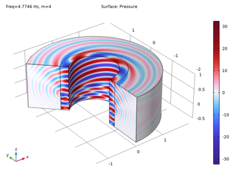
In the Settings window for 3D Plot Group, type Near Field Pressure 2D Revolved in the Label text field.
3
Locate the Data section. From the Dataset list, choose Revolution 2D 2.
Surface 1
1
Right-click Near Field Pressure 2D Revolved and choose Surface.
The circumferential behavior is automatically represented as you defined the Azimuthal mode number in the revolved solution dataset.
2
In the Settings window for Surface, locate the Expression section.
3
In the Expression text field, type ae.p.
4
Locate the Coloring and Style section. From the Color table list, choose Wave.
5
From the Scale list, choose Linear symmetric.
6
In the Near Field Pressure 2D Revolved toolbar, click  Plot.