PDF

Generic 711 Coupler — An Occluded Ear-Canal Simulator
Introduction
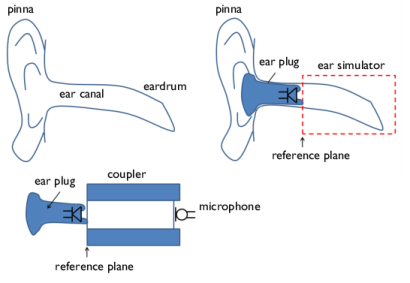
This is a model of a 711 coupler1, an occluded ear-canal simulator that follows the specifications given in the IEC 60318-4 international standard (Ref. 1). A coupler is a device for measuring the acoustic output of sound sources with a calibrated microphone. The microphone is coupled to the source by a cavity of known shape and volume (see Figure 1 bottom). The 711 coupler approximates the acoustic transfer impedance of the inner part of the ear canal from the tip of an ear plug (ear insert or ear mold) located at the reference plane to the eardrum (see Figure 1 top right). It is thus a device that is intended to have the same acoustic properties as the average occluded human ear-canal and eardrum system, approximately from the second bend in the ear canal to the eardrum. The 711 coupler is intended for measurements of hearing aids and earphones that are coupled to the ear by means of an insert earphone.
Figure 1: (upper left) sketch of the ear with pinna, ear canal, and eardrum, (upper right) ear canal occluded by an earplug with a loudspeaker, the occluded-ear canal is the part that the coupler is intended to model, (bottom) ear plug placed at the reference plane of the acoustic coupler including the location of the recording microphone.
Using a coupler for measurement of the acoustic response enables standardized measurements and comparisons. Coupler measurements on ear-canal simulators are also often used for prototype development and testing. Such measurements do, however, not include leakage between ear mold and ear canal. As the coupler represents a normal average human ear it does not mimic the large acoustic performance variations that exist between individual ears (see for example, Ref. 2).
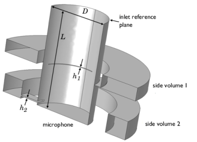
Figure 2: Sketch of the geometry used in the model (cut in half due to symmetry). The main volume is a cylinder of length L and diameter D. The two side volumes are attached to the main volume via slender slits of height h1 and h2.
Model Definition
Geometry
The coupler is made of hard nonporous material and it is terminated at one end by a measurement microphone. This end corresponds to the eardrum (the tympanic membrane) and the measured microphone pressure should correspond the to that perceived by the eardrum. The human eardrum has a nontrivial acoustic behavior (see Ref. 3); the coupler has to account for
1
2
In order for the coupler to do this it is constructed as a main cylinder of length L and diameter D with two attached side volumes, see Figure 2. The side volumes are connected to the main volume via shallow slits of height h1 and h2. The coupler geometry meets the requirements of the IEC 60318-4 international standard (Ref. 1) and besides certain details corresponds to the Brüel & Kjær Ear Simulator Type 4157.
The inclusion of the side volumes and the slits is necessary to mimic the complex eardrum mechanical losses using an acoustic system. In the coupler the losses are mainly due to the high thermal and viscous damping in the slits. The diameter D of the main cylinder is given by the standard and is 7.5 mm. The length of the cylinder is prescribed by the IEC standard to be such as to produce a half-wavelength resonance at around 13.5 kHz. In this model L = 12.5 mm, which gives a resonance at 13.8 kHz. The slit heights are h1 = 69 μm and h2 = 170 μm.
Thermoviscous acoustics
As the thermal and viscous losses are important in the slits the finite element model is set up in COMSOL using two different methods; a model using Thermoviscous Acoustics, Frequency Domain interface and a model with Pressure Acoustics, Frequency Domain interface and the Narrow Region Acoustics feature to account for the losses in the slits. This enables the direct inclusion and modeling of the thermal and viscous losses in the slits. The losses arise in the viscous and thermal boundary layers that are characterized by the length scales:
(1)
Where ω is the angular frequency, μ is the dynamic viscosity, k is the coefficient of thermal conduction, ρ is density, and Cp is the specific heat at constant pressure. Using air properties both layers will have roughly the same length for a given frequency. In the modeled frequency range, from 100 Hz to 20 kHz, this yields length scales from 220 μm to 15 μm (for air at 23° C). Thermal and viscous losses are hence important in most of the frequency range when comparing these length scales to the slit heights. However, they need not be included in the main cylinder and the side volumes, where pressure acoustics may be used. The pressure acoustics and the thermoviscous acoustics domains are coupled using the built in Acoustics-Thermoviscous Acoustics Boundary multiphysics coupling found under the Multiphysics node in the model tree.
Coupler Characterization
The 711 coupler is characterized in the IEC 60318-4 standard in terms of its transfer impedance Ztrans and the microphone response L0 (for a constant volume displacement source):
(2)
where Qin is the volume flow rate at the inlet reference plane, pmic is the root mean square (rms) pressure at the measurement microphone, pref is a reference pressure (here the rms pressure at 500 Hz), and Lref is the corresponding reference level. The transfer impedance of a coupler is easily measured using, for example, a microphone as a sound source (it has a high output impedance and thus a nearly constant Qin). Moreover, the pressure is directly determined by the measurement microphone. In a real ear, Ztrans is somewhat more complicated to measure because it requires the insertion of a probe tube into the ear to measure pmic (now the pressure at the eardrum). The transfer impedance and microphone response are specified in the frequency range 100 Hz to 10 kHz. Above 10 kHz, the 711 coupler does not simulate a human ear.
Generally, to mimic an ear with a coupler one should require both systems to have the same two-port parameters. These are four parameters that relate pressure and volume velocity at the inlet and outlet. If only the acoustic input load and the pressure at the eardrum are of interest, the transfer impedance characterizes the coupler together with the input impedance Zin. The latter is defined as
(3)
where pin is the pressure at the inlet reference plane. Note that it is important to retain the sign of the velocity when computing Qin, in this case such that you look “into” the coupler from the outside. The quantity exists as a predefined postprocessing variable on displacement, velocity, and acceleration boundary conditions in the pressure acoustics interface. The relevant variable acpr.Zac (the acoustic impedance) can be evaluated on surfaces. In systems with, for example, one symmetry its value needs to be divided with 2 (to account for the full area). The specific impedance on the boundary is named acpr.Zi.
Modeling an acoustic coupler is of interest for design and for optimizing the acoustic response with respect to different input systems (see for example Ref. 5). The coupler cannot always be modeled as a simple acoustic load (impedance). Interactions may exist between the sound source outlets (hearing aid ear-mold or earplug) and the coupler acoustics. Nonplane waves may, for example, propagate into the coupler.
Boundary Conditions
At the inlet reference plane, a constant volume source is applied by specifying the inward normal displacement dn of the boundary
(4)
where d0 is the sound source displacement.
At the location of the measurement microphone, an impedance corresponding to the mechanical properties of a Brüel & Kjær 4192 microphone is specified (see Ref. 4 pp 6–18). The impedance is given by
(5)
where Cmic = 0.62·1013 m5/N is the acoustic compliance, Rmic = 119·106 Ns/m5 is the acoustic resistance, and Lmic = 710 kg/m4 is the acoustic mass. This is modeled using the built-in RCL option in the impedance boundary condition.
To reduce the model size, model only half of the geometry and use symmetry conditions on both the pressure acoustic and thermoviscous acoustic domains.
Results and Discussion
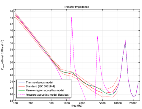
Figure 3 depicts the transfer impedance for the system as a function of frequency. The modeled system is seen to comply well with the IEC standard curve.
Figure 3: Transfer impedance as function of frequency for the thermoviscous model (blue line), the IEC standard curve (red line) including upper and lower tolerances (red dotted line), the system modeled through narrow region acoustics (green line) and the lossless pressure acoustics approach (dotted dark green line).
Also evident from the graph is that it is important to use thermoviscous acoustics to model such acoustic systems with small geometrical dimensions. The narrow region acoustics approach is in good agreement with the thermoviscous model results, showing that for some simple waveguide geometries (slits, rectangular and circular ducts of constant cross-section) the Narrow Region Acoustics feature can reduce substantially the complexity of the model while maintaining accuracy. In the frequency range where the acoustic boundary-layer thickness is comparable to the small slit heights, the lossless model is completely off because all the resonances are undamped. Above about 10 kHz the thermal and viscous losses in the slits are much less pronounced and the only system losses are due to the RCL impedance condition representing the microphone.
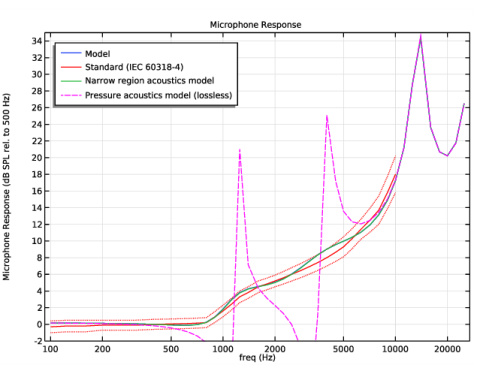
Figure 4 depicts the microphone response measured for a constant displacement source, again comparing model results to the IEC standard and the lossless model.
Figure 4: Microphone response as function of frequency for the thermoviscous model (blue line), the IEC standard curve (red line) including upper and lower tolerances (red dotted line), the system modeled through narrow region acoustics (green line) and the lossless pressure acoustics approach (dotted dark green line).
The input impedance of the system derived at the reference plane is shown in Figure 5 where the model results are compared to the results of the fully lossless model.
Figure 5: Input impedance as function of frequency for the thermoviscous model (blue line), the system modeled with narrow region acoustics (green line), and the lossless pressure acoustics approach (red line).
Figure 6, Figure 7, and Figure 8 depict the pressure distribution inside the 711 coupler at frequencies of 25 kHz, 14 kHz, and 900 Hz, respectively. The first figure represents the standing wave mode inside the inner tube and the second figure the half wave standing mode. The last figure represents a Helmholtz-like resonance in the lower side volume.
Figure 6: Instantaneous pressure distribution at f = 25 kHz.
Figure 7: Instantaneous pressure distribution at f = 14 kHz.
Figure 8: Instantaneous pressure distribution at f = 900Hz.
The losses in the thermoviscous model are shown in Figure 9 normalized to the total acoustic power in the system. The plot shows the effect of the different slits as the frequency increases, and how the microphone starts absorbing energy above 5 kHz.
Figure 9: Normalized losses in the thermoviscous model.
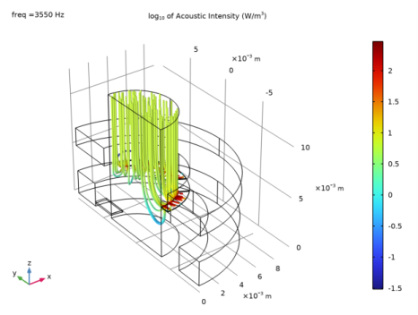
The same conclusion could be drawn by plotting the streamline of acoustic intensity at the frequencies of the peak losses for each of the systems. Figure 10, Figure 11, and Figure 12 show the streamline of acoustic intensity at 800 Hz, 3,550 Hz and 18,000 Hz, matching the peak losses in the bottom slit, the top slit and the microphone respectively.
Figure 10: streamline of acoustic intensity at 800 Hz
Figure 11: Streamline of acoustic intensity at 3,550 Hz
Figure 12: Streamline of acoustic intensity at 18,000 Hz
References
1. IEC 60318-4, Electroacoustics — Simulators of human head and ear — Part 4: Occluded-ear simulator for the measurement of earphones coupled to the ear by means of ear inserts, edition 1.0, 2010.
2. M.R. Stinson and B.W. Lawton, “Specification of the geometry of the human ear canal for the prediction of sound-pressure level distribution,” J. Acoust. Soc. Am., vol. 85, pp. 2492–2503, 1989.
3. M.R. Stinson, “The spatial distribution of sound pressure within scaled replicas of the human ear canal,” J. Acoust. Soc. Am., vol. 78, no. 5, pp. 1596–1602, 1985.
4. Brüel and Kjær, Microphone Handbook: For the Falcon Range Microphone Products, Technical Documentation, 1995.
5. B.L. Zhang, S. Jønsson, A. Schuhmacher, and L.B. Nielsen, A Combined BEM/FEM Acoustic Model of an Occluded Ear Simulator, InterNoise 2004, Prague, Czech Republic, 2004.
Application Library path: Acoustics_Module/Tutorials,_Thermoviscous_Acoustics/generic_711_coupler
Modeling Instructions
From the File menu, choose New.
New
In the New window, click  Model Wizard.
Model Wizard
1
In the Model Wizard window, click  3D.
2
In the Select Physics tree, select Acoustics>Pressure Acoustics>Pressure Acoustics, Frequency Domain (acpr).
3
Click Add.
4
In the Select Physics tree, select Acoustics>Thermoviscous Acoustics>Thermoviscous Acoustics, Frequency Domain (ta).
5
Click Add.
6
Global Definitions
Load the parameters for the model. The list of parameters includes the maximal mesh size, the microphone impedance parameters, and other reference values.
Parameters 1
1
In the Model Builder window, under Global Definitions click Parameters 1.
2
In the Settings window for Parameters, locate the Parameters section.
3
Click  Load from File.
4
To make the data for the transfer impedance and microphone response available in the model, create six interpolation functions. The data are located in two text files and comprise the nominal values as well as upper and lower tolerances as defined in the IEC 60318-4 standard (Table 1 and Table B.1 in Ref. 1).
Interpolation 1 (int1)
1
In the Home toolbar, click  Functions and choose Global>Interpolation.
2
In the Settings window for Interpolation, locate the Definition section.
3
From the Data source list, choose File.
4
Click  Browse.
5
6
In the Number of arguments text field, type 1.
7
Click  Import.
8
Find the Functions subsection. In the table, enter the following settings:
Interpolation 2 (int2)
1
In the Home toolbar, click  Functions and choose Global>Interpolation.
2
In the Settings window for Interpolation, locate the Definition section.
3
From the Data source list, choose File.
4
Click  Browse.
5
6
In the Number of arguments text field, type 1.
7
Click  Import.
8
Find the Functions subsection. In the table, enter the following settings:
Geometry 1
Import the model geometry from file by following these steps.
Import 1 (imp1)
1
In the Home toolbar, click  Import.
2
In the Settings window for Import, locate the Import section.
3
Click  Browse.
4
5
Click  Import.
6
Click the  Zoom Extents button in the Graphics toolbar.
The figure below shows the model geometry.
Definitions
Load a set of variables that define the microphone impedance (Equation 5), the acoustic transfer impedance (Equation 2), and the acoustic input impedance (Equation 4) from a file. Add operators to integrate values across the inlet plane, the microphone plane and the slit domains.
Variables 1
1
In the Home toolbar, click  Variables and choose Local Variables.
2
In the Settings window for Variables, locate the Variables section.
3
Click  Load from File.
4
Integration 1 (intop1)
1
In the Definitions toolbar, click  Nonlocal Couplings and choose Integration.
2
In the Settings window for Integration, type intop_in in the Operator name text field.
3
Locate the Source Selection section. From the Geometric entity level list, choose Boundary.
4
Integration 2 (intop2)
1
In the Definitions toolbar, click  Nonlocal Couplings and choose Integration.
2
In the Settings window for Integration, type intop_mic in the Operator name text field.
3
Locate the Source Selection section. From the Geometric entity level list, choose Boundary.
4
Integration 3 (intop3)
1
In the Definitions toolbar, click  Nonlocal Couplings and choose Integration.
2
In the Settings window for Integration, type intop_top_slit in the Operator name text field.
3
Integration 4 (intop4)
1
In the Definitions toolbar, click  Nonlocal Couplings and choose Integration.
2
In the Settings window for Integration, type intop_bottom_slit in the Operator name text field.
3
Next, make selections of different parts of the geometry to ease the subsequent application of boundary conditions. Then proceed and set up the acoustic model and the boundary conditions.
Pressure Acoustics (lossless)
1
In the Definitions toolbar, click  Explicit.
2
3
In the Settings window for Explicit, type Pressure Acoustics (lossless) in the Label text field.
Thermoviscous Acoustics
1
In the Definitions toolbar, click  Explicit.
2
3
In the Settings window for Explicit, type Thermoviscous Acoustics in the Label text field.
Symmetry
1
In the Definitions toolbar, click  Explicit.
2
In the Settings window for Explicit, locate the Input Entities section.
3
From the Geometric entity level list, choose Boundary.
4
5
In the Label text field, type Symmetry.
Add Material
1
In the Home toolbar, click  Add Material to open the Add Material window.
2
Go to the Add Material window.
3
4
Click Add to Component in the window toolbar.
5
In the Home toolbar, click  Add Material to close the Add Material window.
Pressure Acoustics, Frequency Domain (acpr)
1
In the Model Builder window, under Component 1 (comp1) click Pressure Acoustics, Frequency Domain (acpr).
2
In the Settings window for Pressure Acoustics, Frequency Domain, locate the Domain Selection section.
3
From the Selection list, choose Pressure Acoustics (lossless).
Pressure Acoustics 1
1
In the Model Builder window, under Component 1 (comp1)>Pressure Acoustics, Frequency Domain (acpr) click Pressure Acoustics 1.
2
In the Settings window for Pressure Acoustics, locate the Model Input section.
3
In the T text field, type Tref.
Symmetry 1
1
In the Physics toolbar, click  Boundaries and choose Symmetry.
2
In the Settings window for Symmetry, locate the Boundary Selection section.
3
From the Selection list, choose Symmetry.
Normal Displacement 1
1
In the Physics toolbar, click  Boundaries and choose Normal Displacement.
2
3
In the Settings window for Normal Displacement, locate the Normal Displacement section.
4
In the dn text field, type d0.
Impedance 1
1
In the Physics toolbar, click  Boundaries and choose Impedance.
2
3
In the Settings window for Impedance, locate the Impedance section.
4
From the Impedance model list, choose RCL.
5
In the Rac text field, type Rmic.
6
In the Cac text field, type Cmic.
7
In the Lac text field, type Lmic.
Thermoviscous Acoustics, Frequency Domain (ta)
Thermoviscous Acoustics Model 1
1
In the Model Builder window, under Component 1 (comp1)>Thermoviscous Acoustics, Frequency Domain (ta) click Thermoviscous Acoustics Model 1.
2
In the Settings window for Thermoviscous Acoustics Model, locate the Model Input section.
3
In the T0 text field, type Tref.
4
In the Model Builder window, click Thermoviscous Acoustics, Frequency Domain (ta).
5
In the Settings window for Thermoviscous Acoustics, Frequency Domain, locate the Domain Selection section.
6
From the Selection list, choose Thermoviscous Acoustics.
Symmetry 1
1
In the Physics toolbar, click  Boundaries and choose Symmetry.
2
In the Settings window for Symmetry, locate the Boundary Selection section.
3
From the Selection list, choose Symmetry.
Next, create and set up the multiphysics coupling between the pressure acoustics domain and the thermoviscous acoustics domain.
Multiphysics
Acoustic-Thermoviscous Acoustic Boundary 1 (atb1)
1
In the Physics toolbar, click  Multiphysics Couplings and choose Boundary>Acoustic-Thermoviscous Acoustic Boundary.
2
In the Settings window for Acoustic-Thermoviscous Acoustic Boundary, locate the Boundary Selection section.
3
From the Selection list, choose All boundaries.
Add another Pressure Acoustics, Frequency Domain physics interface. You will use this to illustrate the effect of thermoviscous acoustics in the slit channels by comparing to a solution of the same problem using regular pressure acoustics and narrow region acoustics here.
Add Physics
1
In the Physics toolbar, click  Add Physics to open the Add Physics window.
2
Go to the Add Physics window.
3
In the tree, select Acoustics>Pressure Acoustics>Pressure Acoustics, Frequency Domain (acpr).
4
Click Add to Component 1 in the window toolbar.
5
In the Physics toolbar, click  Add Physics to close the Add Physics window.
Pressure Acoustics, Frequency Domain 2 (acpr2)
1
In the Settings window for Pressure Acoustics, Frequency Domain, locate the Domain Selection section.
2
From the Selection list, choose Thermoviscous Acoustics.
Pressure Acoustics 1
1
In the Model Builder window, under Component 1 (comp1)>Pressure Acoustics, Frequency Domain 2 (acpr2) click Pressure Acoustics 1.
2
In the Settings window for Pressure Acoustics, locate the Model Input section.
3
In the T text field, type Tref.
Symmetry 1
1
In the Physics toolbar, click  Boundaries and choose Symmetry.
2
In the Settings window for Symmetry, locate the Boundary Selection section.
3
From the Selection list, choose Symmetry.
Couple the two pressure acoustics interfaces together. The simplest approach is to give the dependent variable, the pressure, the same name p. Note that this approach is only valid when coupling identical physics.
4
In the Model Builder window, click Pressure Acoustics, Frequency Domain 2 (acpr2).
5
In the Settings window for Pressure Acoustics, Frequency Domain, click to expand the Dependent Variables section.
6
In the Pressure text field, type p.
Now, add the narrow region acoustics features that will introduce losses in the narrow slits.
Narrow Region Acoustics 1
1
In the Physics toolbar, click  Domains and choose Narrow Region Acoustics.
2
3
In the Settings window for Narrow Region Acoustics, locate the Duct Properties section.
4
From the Duct type list, choose Rectangular duct.
5
In the W text field, type 2230 [um].
6
In the H text field, type 170 [um].
In this case, the slit is well approximated by a rectangular duct. The dimensions of the slit in the vertical direction and the total horizontal dimension are used to compute an equivalent loss instead of solving the set of thermoviscous equations.
Narrow Region Acoustics 2
1
In the Physics toolbar, click  Domains and choose Narrow Region Acoustics.
2
3
In the Settings window for Narrow Region Acoustics, locate the Duct Properties section.
4
From the Duct type list, choose Slit.
5
In the h text field, type 69[um].
As this slit has a very large aspect ratio, it is well approximated by a slit. In this case, only one of the dimensions of the slit is used to obtain the equivalent losses.
In this model, the mesh is set up manually. Proceed by directly adding the desired mesh component.
Start using a swept mapped mesh in the slits and then add a tetrahedral mesh in the remaining domains.
Mesh 1
Mapped 1
1
In the Mesh toolbar, click  Boundary and choose Mapped.
2
Distribution 1
1
Right-click Mapped 1 and choose Distribution.
2
3
In the Settings window for Distribution, locate the Distribution section.
4
In the Number of elements text field, type 4.
Distribution 2
1
In the Model Builder window, right-click Mapped 1 and choose Distribution.
2
3
In the Settings window for Distribution, locate the Distribution section.
4
In the Number of elements text field, type 25.
Distribution 3
1
Right-click Mapped 1 and choose Distribution.
2
3
In the Settings window for Distribution, locate the Distribution section.
4
In the Number of elements text field, type 36.
Distribution 4
1
Right-click Mapped 1 and choose Distribution.
2
3
In the Settings window for Distribution, locate the Distribution section.
4
In the Number of elements text field, type 8.
Distribution 5
1
Right-click Mapped 1 and choose Distribution.
2
3
In the Settings window for Distribution, locate the Distribution section.
4
In the Number of elements text field, type 7.
Distribution 6
1
Right-click Mapped 1 and choose Distribution.
2
3
In the Settings window for Distribution, locate the Distribution section.
4
In the Number of elements text field, type 6.
5
Click  Build Selected.
The mapped mesh on the upper side of the slits looks like that in the figure above (switch to wireframe rendering).
Now, proceed to sweep the mesh in the slits.
Size
1
In the Model Builder window, under Component 1 (comp1)>Mesh 1 click Size.
2
In the Settings window for Size, locate the Element Size section.
3
Click the Custom button.
4
Locate the Element Size Parameters section. In the Maximum element size text field, type Lmax.
5
In the Minimum element size text field, type 0.2[mm].
Swept 1
1
In the Mesh toolbar, click  Swept.
2
In the Settings window for Swept, locate the Domain Selection section.
3
From the Geometric entity level list, choose Domain.
4
Distribution 1
1
Right-click Swept 1 and choose Distribution.
2
In the Settings window for Distribution, locate the Distribution section.
3
In the Number of elements text field, type 3.
4
Click  Build Selected.
5
In the Model Builder window, right-click Mesh 1 and choose Build Selected.
Free Tetrahedral 1
In the Mesh toolbar, click  Free Tetrahedral.
Size 1
1
Right-click Free Tetrahedral 1 and choose Size.
2
In the Settings window for Size, locate the Geometric Entity Selection section.
3
From the Geometric entity level list, choose Boundary.
4
5
Locate the Element Size section. Click the Custom button.
6
Locate the Element Size Parameters section. Select the Maximum element size check box.
7
8
Click  Build All.
The mesh should look similar to that shown in the figure below.
Add Study
1
In the Home toolbar, click  Add Study to open the Add Study window.
2
Go to the Add Study window.
3
Find the Studies subsection. In the Select Study tree, select General Studies>Frequency Domain.
4
Click Add Study in the window toolbar.
5
In the Home toolbar, click  Add Study to close the Add Study window.
Turn off the generation of the default plots and create your own. Leave this option on to have the default plot of Pressure Acoustics and Thermoviscous Acoustics generated.
Study 1 - Thermoviscous Model
1
In the Model Builder window, click Study 1.
2
In the Settings window for Study, type Study 1 - Thermoviscous Model in the Label text field.
3
Locate the Study Settings section. Clear the Generate default plots check box.
Step 1: Frequency Domain
1
In the Model Builder window, under Study 1 - Thermoviscous Model click Step 1: Frequency Domain.
2
In the Settings window for Frequency Domain, locate the Study Settings section.
3
Click  Range.
4
In the Range dialog box, choose ISO preferred frequencies from the Entry method list.
5
In the Start frequency text field, type 100.
6
In the Stop frequency text field, type 25000.
7
From the Interval list, choose 1/6 octave.
8
Click Replace.
9
In the Settings window for Frequency Domain, locate the Physics and Variables Selection section.
10
Select the Modify model configuration for study step check box.
11
In the tree, select Component 1 (Comp1)>Pressure Acoustics, Frequency Domain 2 (Acpr2).
12
Click  Disable in Model.
13
In the Home toolbar, click  Compute.
Note that the computation may take several minutes.
Add a second study to solve the model with narrow region acoustics. Disable thermoviscous acoustics and enable the second pressure acoustics model, in this way the system will use the narrow region acoustics. The results from the second study are stored in a separate dataset. Compare this second solution to the model that includes the complete set of equations.
Add Study
1
In the Home toolbar, click  Add Study to open the Add Study window.
2
Go to the Add Study window.
3
Find the Studies subsection. In the Select Study tree, select General Studies>Frequency Domain.
4
Find the Physics interfaces in study subsection. In the table, clear the Solve check box for Thermoviscous Acoustics, Frequency Domain (ta).
5
Click Add Study in the window toolbar.
6
In the Home toolbar, click  Add Study to close the Add Study window.
Study 2 - Narrow Region Acoustics
1
In the Model Builder window, click Study 2.
2
In the Settings window for Study, type Study 2 - Narrow Region Acoustics in the Label text field.
3
Locate the Study Settings section. Clear the Generate default plots check box.
Step 1: Frequency Domain
1
In the Model Builder window, under Study 2 - Narrow Region Acoustics click Step 1: Frequency Domain.
2
In the Settings window for Frequency Domain, locate the Study Settings section.
3
Click  Range.
4
In the Range dialog box, choose ISO preferred frequencies from the Entry method list.
5
In the Start frequency text field, type 100.
6
In the Stop frequency text field, type 25000.
7
From the Interval list, choose 1/6 octave.
8
Click Replace.
Make some small changes to the default solver to use a fully coupled approach when solving the two pressure acoustics physics together.
Solution 2 (sol2)
1
In the Study toolbar, click  Show Default Solver.
2
In the Model Builder window, expand the Solution 2 (sol2) node.
3
In the Model Builder window, expand the Study 2 - Narrow Region Acoustics>Solver Configurations>Solution 2 (sol2)>Stationary Solver 1 node.
4
Right-click Study 2 - Narrow Region Acoustics>Solver Configurations>Solution 2 (sol2)>Stationary Solver 1 and choose Fully Coupled.
Select the direct solver that uses MUMPS, or change the solver in the selected Direct 1 solver.
5
In the Settings window for Fully Coupled, locate the General section.
6
From the Linear solver list, choose Direct.
7
In the Study toolbar, click  Compute.
Now create a last step where a pressure acoustics (Lossless) model is analyzed. To do this, you need to turn off the narrow region acoustics domains in the second pressure acoustics physics.
Add Study
1
In the Study toolbar, click  Add Study to open the Add Study window.
2
Go to the Add Study window.
3
Find the Studies subsection. In the Select Study tree, select General Studies>Frequency Domain.
4
Find the Physics interfaces in study subsection. In the table, clear the Solve check box for Thermoviscous Acoustics, Frequency Domain (ta).
5
Find the Multiphysics couplings in study subsection. In the table, clear the Solve check box for Acoustic-Thermoviscous Acoustic Boundary 1 (atb1).
6
Click Add Study in the window toolbar.
7
In the Study toolbar, click  Add Study to close the Add Study window.
Study 3 - Pressure Acoustics
1
In the Model Builder window, click Study 3.
2
In the Settings window for Study, type Study 3 - Pressure Acoustics in the Label text field.
3
Locate the Study Settings section. Clear the Generate default plots check box.
4
Clear the Generate convergence plots check box.
Step 1: Frequency Domain
1
In the Model Builder window, under Study 3 - Pressure Acoustics click Step 1: Frequency Domain.
2
In the Settings window for Frequency Domain, locate the Study Settings section.
3
Click  Range.
4
In the Range dialog box, choose ISO preferred frequencies from the Entry method list.
5
In the Start frequency text field, type 100.
6
In the Stop frequency text field, type 25000.
7
From the Interval list, choose 1/6 octave.
8
Click Replace.
9
In the Settings window for Frequency Domain, locate the Physics and Variables Selection section.
10
Select the Modify model configuration for study step check box.
11
In the tree, select Component 1 (Comp1)>Pressure Acoustics, Frequency Domain 2 (Acpr2)>Narrow Region Acoustics 1 and Component 1 (Comp1)>Pressure Acoustics, Frequency Domain 2 (Acpr2)>Narrow Region Acoustics 2.
12
Click  Disable.
With this, the narrow region acoustics will not be considered in the analysis, so the model becomes lossless.
Make some small changes to the default solver to use a fully coupled approach when solving the two pressure acoustics physics together.
13
Right-click Study 3 - Pressure Acoustics>Step 1: Frequency Domain and choose Get Initial Value for Step.
Solver Configurations
In the Model Builder window, expand the Study 3 - Pressure Acoustics>Solver Configurations node.
Solution 3 (sol3)
1
In the Model Builder window, expand the Study 3 - Pressure Acoustics>Solver Configurations>Solution 3 (sol3)>Stationary Solver 1 node.
2
Right-click Stationary Solver 1 and choose Fully Coupled.
3
Right-click Direct and choose Enable.
4
In the Settings window for Direct, click  Compute.
Results
First, create plots of the pressure distribution inside the coupler. Then move on to plotting the transfer impedance, input impedance, and the microphone response.
Acoustic Pressure
1
In the Home toolbar, click  Add Plot Group and choose 3D Plot Group.
2
In the Settings window for 3D Plot Group, type Acoustic Pressure in the Label text field.
Volume 1
1
Right-click Acoustic Pressure and choose Volume.
2
In the Settings window for Volume, locate the Coloring and Style section.
3
From the Color table list, choose Wave.
Volume 2
1
In the Model Builder window, right-click Acoustic Pressure and choose Volume.
2
In the Settings window for Volume, locate the Expression section.
3
In the Expression text field, type ta.p_t.
4
Click to expand the Title section. From the Title type list, choose None.
5
Click to expand the Inherit Style section. From the Plot list, choose Volume 1.
6
In the Acoustic Pressure toolbar, click  Plot.
The plot should look like Figure 6. To create Figure 7, and Figure 8 change the evaluation frequency to 14000 Hz and 900 Hz, respectively.
Next, generate a plot to show the streamline of the acoustic energy and investigate where the losses of the model are depending on the frequency.
Streamline - Acoustic Intensity
1
In the Home toolbar, click  Add Plot Group and choose 3D Plot Group.
2
In the Settings window for 3D Plot Group, locate the Data section.
3
From the Parameter value (freq (Hz)) list, choose 18000.
4
In the Label text field, type Streamline - Acoustic Intensity.
5
Click to expand the Title section. From the Title type list, choose Manual.
6
In the Title text area, type log<sub>10</sub> of Acoustic Intensity (W/m<sup>3</sup>).
7
In the Parameter indicator text field, type freq =eval(acpr.freq) Hz.
Streamline 1
1
Right-click Streamline - Acoustic Intensity and choose Streamline.
2
In the Settings window for Streamline, locate the Expression section.
3
In the X component text field, type if(isnan(acpr.p_t),ta.Ix,acpr.Ix).
4
In the Y component text field, type if(isnan(acpr.p_t),ta.Iy,acpr.Iy).
5
In the Z component text field, type if(isnan(acpr.p_t),ta.Iz,acpr.Iz).
6
7
Locate the Streamline Positioning section. In the Number text field, type 100.
8
Locate the Coloring and Style section. Find the Line style subsection. From the Type list, choose Tube.
Color Expression 1
1
Right-click Streamline 1 and choose Color Expression.
2
In the Settings window for Color Expression, locate the Expression section.
3
In the Expression text field, type if(isnan(acpr.p_t),log10(ta.I_mag),log10(acpr.I_mag)).
4
In the Streamline - Acoustic Intensity toolbar, click  Plot.
The plot should look like Figure 10. To create Figure 11, and Figure 12 change the evaluation frequency to 3550 Hz and 800 Hz, respectively.
Plot the transfer impedance for the thermoviscous, the narrow region acoustics model, and the pressure acoustics (lossless) model as well as the curves given by the standard Figure 3.
Transfer Impedance
1
In the Home toolbar, click  Add Plot Group and choose 1D Plot Group.
2
In the Settings window for 1D Plot Group, type Transfer Impedance in the Label text field.
3
Click to expand the Title section. From the Title type list, choose Label.
4
Locate the Plot Settings section. Select the y-axis label check box.
5
In the associated text field, type Z<sub>trans</sub> (dB rel. 1MPa·s/m<sup>3</sup>).
6
Locate the Legend section. From the Position list, choose Lower left.
Global 1
1
Right-click Transfer Impedance and choose Global.
2
In the Settings window for Global, locate the y-Axis Data section.
3
Global 2
1
In the Model Builder window, right-click Transfer Impedance and choose Global.
2
In the Settings window for Global, locate the y-Axis Data section.
3
4
Click to expand the Coloring and Style section. From the Color list, choose Red.
5
Locate the Data section. From the Dataset list, choose Study 1 - Thermoviscous Model/Solution 1 (sol1).
Only plot the curves given by the IEC standard in the range from 100 Hz to 10 kHz, where they are defined.
6
From the Parameter selection (freq) list, choose From list.
7
In the Parameter values list, choose values from 100 to 10000.
8
In the Transfer Impedance toolbar, click  Plot.
9
Click the  x-Axis Log Scale button in the Graphics toolbar.
Global 3
1
Right-click Global 2 and choose Duplicate.
2
In the Settings window for Global, locate the y-Axis Data section.
3
4
Locate the Coloring and Style section. Find the Line style subsection. From the Line list, choose Dotted.
5
Click to expand the Legends section. Clear the Show legends check box.
Global 4
1
In the Model Builder window, under Results>Transfer Impedance right-click Global 1 and choose Duplicate.
2
In the Settings window for Global, locate the Data section.
3
From the Dataset list, choose Study 2 - Narrow Region Acoustics/Solution 2 (sol2).
4
Locate the y-Axis Data section. In the table, enter the following settings:
5
In the Transfer Impedance toolbar, click  Plot.
Global 5
1
Right-click Global 4 and choose Duplicate.
2
In the Settings window for Global, locate the Data section.
3
From the Dataset list, choose Study 3 - Pressure Acoustics/Solution 3 (sol3).
4
Locate the y-Axis Data section. In the table, enter the following settings:
5
Locate the Coloring and Style section. From the Color list, choose Magenta.
6
Find the Line style subsection. From the Line list, choose Dashed.
7
In the Transfer Impedance toolbar, click  Plot.
Transfer Impedance
1
In the Model Builder window, click Transfer Impedance.
2
In the Settings window for 1D Plot Group, locate the Axis section.
3
Select the Manual axis limits check box.
4
In the y minimum text field, type 18.
5
In the Transfer Impedance toolbar, click  Plot.
Microphone Response
1
Right-click Transfer Impedance and choose Duplicate.
Proceed to reproduce the plot of the microphone response Figure 4.
2
In the Settings window for 1D Plot Group, type Microphone Response in the Label text field.
3
Locate the Plot Settings section. In the y-axis label text field, type Microphone Response (dB SPL rel. to 500 Hz).
4
Locate the Legend section. From the Position list, choose Upper left.
Global 1
1
In the Model Builder window, expand the Microphone Response node, then click Global 1.
2
In the Settings window for Global, locate the y-Axis Data section.
3
Global 2
1
In the Model Builder window, click Global 2.
2
In the Settings window for Global, locate the y-Axis Data section.
3
Global 3
1
In the Model Builder window, click Global 3.
2
In the Settings window for Global, locate the y-Axis Data section.
3
Global 4
1
In the Model Builder window, click Global 4.
2
In the Settings window for Global, locate the y-Axis Data section.
3
Global 5
1
In the Model Builder window, click Global 5.
2
In the Settings window for Global, locate the y-Axis Data section.
3
Microphone Response
1
In the Model Builder window, click Microphone Response.
2
In the Settings window for 1D Plot Group, locate the Axis section.
3
In the y minimum text field, type -2.
4
In the y maximum text field, type 35.
5
In the Microphone Response toolbar, click  Plot.
Now, plot the input impedance for the thermoviscous, the narrow region acoustics, and the pressure acoustics model as seen in Figure 5.
Input Impedance
1
In the Home toolbar, click  Add Plot Group and choose 1D Plot Group.
2
In the Settings window for 1D Plot Group, type Input Impedance in the Label text field.
3
Locate the Title section. From the Title type list, choose Label.
4
Locate the Plot Settings section. Select the y-axis label check box.
5
In the associated text field, type Z<sub>in</sub> (dB rel. 1MPa·s/m<sup>3</sup>).
Global 1
1
Right-click Input Impedance and choose Global.
2
In the Settings window for Global, locate the y-Axis Data section.
3
Global 2
1
Right-click Global 1 and choose Duplicate.
2
In the Settings window for Global, locate the Data section.
3
From the Dataset list, choose Study 2 - Narrow Region Acoustics/Solution 2 (sol2).
4
Locate the y-Axis Data section. In the table, enter the following settings:
Global 3
1
Right-click Global 2 and choose Duplicate.
2
In the Settings window for Global, locate the Data section.
3
From the Dataset list, choose Study 3 - Pressure Acoustics/Solution 3 (sol3).
4
Locate the y-Axis Data section. In the table, enter the following settings:
5
Locate the Coloring and Style section. From the Color list, choose Magenta.
6
Find the Line style subsection. From the Line list, choose Dashed.
7
Click the  x-Axis Log Scale button in the Graphics toolbar.
8
In the Input Impedance toolbar, click  Plot.
The plot should look like Figure 5.
Now, generate a plot showing the losses of the model as a function of the frequency.
Normalized Losses
1
In the Home toolbar, click  Add Plot Group and choose 1D Plot Group.
2
In the Settings window for 1D Plot Group, type Normalized Losses in the Label text field.
3
Locate the Title section. From the Title type list, choose Label.
4
Locate the Legend section. From the Position list, choose Upper left.
Global 1
1
Right-click Normalized Losses and choose Global.
2
In the Settings window for Global, locate the y-Axis Data section.
3
4
Click the  x-Axis Log Scale button in the Graphics toolbar.
5
In the Normalized Losses toolbar, click  Plot.
The plot should look like Figure 9.
In the same way as you have created the plot of the pressure distribution (the first 3D plot), by plotting acpr.p_t and ta.p_t together, other acoustic quantities can be depicted. For example, to plot the sound pressure level plot acpr.Lp_t and ta.Lp_t in the same plot. More details, resolved by thermoviscous acoustics, can be plotted inside the slits by, for example, plotting the acoustic temperature variations ta.T_t, the rms velocity ta.v_rms, or the instantaneous velocity ta.v_inst.
 

1
Here 711 are the last digits in the IEC 60711 standard (1981), which is the standard that the current updated IEC 60318-4 replaces. This has given the occluded ear-canal simulator its commonly used name.