|
|
|
|
1
|
|
•
|
|
•
|
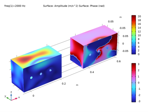
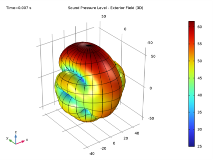
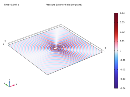
The excitation frequency is taken as 2000 Hz.
|
|
•
|
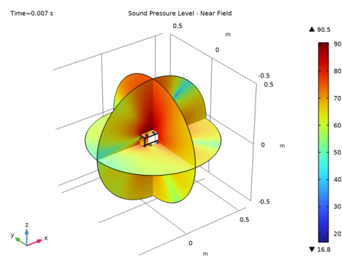
Exterior field results are evaluated at a distance of 2 m from the center.
|
|
1
|
|
2
|
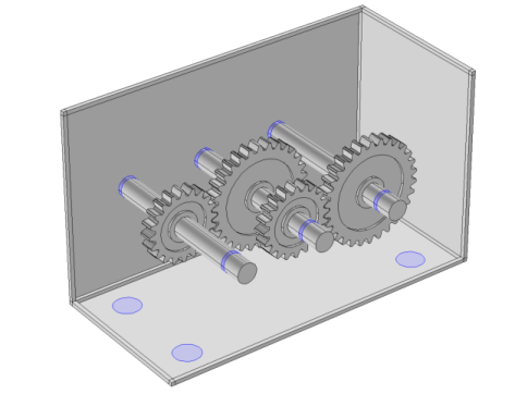
In the Application Libraries window, select Multibody Dynamics Module>Tutorials, Transmission>gear_train in the tree.
|
|
3
|
Click
|
|
1
|
|
2
|
|
1
|
|
2
|
|
3
|
|
4
|
|
5
|
|
6
|
In the Paste Selection dialog box, type 14,38,46,53,65,132,219,220,225,455,456,461,919,920,925 in the Selection text field.
|
|
7
|
Click OK.
|
|
8
|
|
9
|
|
1
|
|
2
|
|
3
|
|
4
|
|
5
|
|
6
|
|
7
|
|
8
|
|
9
|
|
1
|
|
2
|
|
1
|
|
2
|
|
1
|
|
2
|
|
3
|
Click
|
|
4
|
Browse to the model’s Application Libraries folder and double-click the file gear_train_noise.mphbin.
|
|
5
|
Click
|
|
1
|
|
2
|
|
3
|
Click in the Graphics window and then press Ctrl+A to select all objects.
|
|
4
|
|
1
|
|
2
|
|
3
|
|
4
|
|
5
|
|
6
|
|
1
|
|
2
|
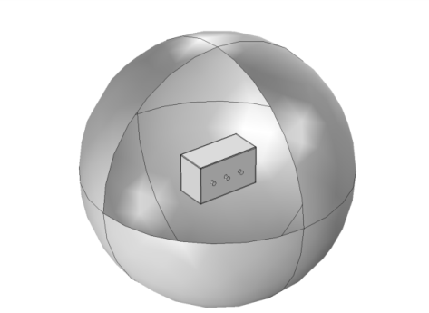
Select the object sph1 only.
|
|
3
|
|
4
|
|
5
|
Select the object csol1 only.
|
|
6
|
|
1
|
|
2
|
|
3
|
|
4
|
Find the Physics interfaces in study subsection. In the table, clear the Solve check boxes for Study 1 - Gear 2D and Study 2 - Gear Train.
|
|
5
|
|
6
|
|
7
|
|
8
|
|
9
|
|
1
|
|
2
|
|
3
|
In the tree, select Built-in>Air.
|
|
4
|
|
5
|
|
1
|
|
2
|
|
3
|
|
5
|
|
6
|
|
1
|
|
2
|
|
3
|
|
4
|
|
5
|
|
6
|
|
1
|
|
2
|
|
3
|
|
4
|
|
5
|
|
6
|
Click
|
|
7
|
|
8
|
Click OK.
|
|
9
|
|
10
|
|
11
|
|
12
|
Click
|
|
13
|
|
14
|
Click OK.
|
|
15
|
|
16
|
|
17
|
|
18
|
|
19
|
In the Dependent variables table, enter the following settings:
|
|
1
|
In the Model Builder window, under Component 3 (comp3)>Boundary ODEs and DAEs (bode) click Distributed ODE 1.
|
|
2
|
|
3
|
|
4
|
|
1
|
|
2
|
|
3
|
|
1
|
|
2
|
|
3
|
|
4
|
|
1
|
|
2
|
|
3
|
|
4
|
|
1
|
|
2
|
|
3
|
|
4
|
|
5
|
In the Show More Options dialog box, in the tree, select the check box for the node Physics>Advanced Physics Options.
|
|
6
|
Click OK.
|
|
7
|
In the Settings window for Exterior Field Calculation, click to expand the Advanced Settings section.
|
|
8
|
|
1
|
|
2
|
|
3
|
Click the Custom button.
|
|
4
|
Locate the Element Size Parameters section. In the Maximum element size text field, type 343[m/s]/f0/5.
|
|
5
|
|
1
|
|
2
|
In the Settings window for Boundary Layer Properties, locate the Geometric Entity Selection section.
|
|
3
|
|
4
|
|
5
|
|
6
|
|
7
|
|
1
|
|
2
|
|
3
|
|
4
|
|
5
|
|
1
|
|
2
|
|
1
|
|
2
|
|
3
|
|
4
|
|
5
|
|
6
|
|
7
|
Locate the Physics and Variables Selection section. In the table, clear the Solve for check boxes for Multibody Dynamics (mbd), Multibody Dynamics 2 (mbd2), and Pressure Acoustics, Frequency Domain (acpr).
|
|
1
|
In the Model Builder window, right-click Study 3 - Acoustics and choose Study Steps>Frequency Domain>Frequency Domain.
|
|
2
|
|
3
|
|
4
|
Locate the Physics and Variables Selection section. In the table, clear the Solve for check boxes for Multibody Dynamics (mbd), Multibody Dynamics 2 (mbd2), and Boundary ODEs and DAEs (bode).
|
|
5
|
Click to expand the Values of Dependent Variables section. Find the Values of variables not solved for subsection. From the Settings list, choose User controlled.
|
|
6
|
|
7
|
|
8
|
|
1
|
|
2
|
|
3
|
|
4
|
|
5
|
|
6
|
|
7
|
|
8
|
|
1
|
|
2
|
|
1
|
In the Model Builder window, right-click Study 3 - Acoustics/Solution 3 (9) (sol3) and choose Selection.
|
|
2
|
|
3
|
|
4
|
|
1
|
In the Model Builder window, expand the Study 3 - Acoustics/Solution 3 (10) (sol3) node, then click Selection.
|
|
2
|
|
3
|
|
4
|
|
5
|
In the Paste Selection dialog box, type 5-7,10-14,16-27,29-39,43-45,48-49,53-55,57,59,67-69,71,73-96 in the Selection text field.
|
|
6
|
Click OK.
|
|
1
|
|
2
|
|
3
|
|
4
|
Locate the Parameter Bounds section. Find the First parameter subsection. In the Minimum text field, type -2.
|
|
5
|
|
6
|
|
7
|
|
8
|
|
9
|
|
10
|
|
11
|
|
1
|
|
2
|
|
3
|
|
4
|
|
5
|
In the Rename 3D Plot Group dialog box, type Housing normal acceleration: amplitude and phase in the New label text field.
|
|
6
|
Click OK.
|
|
1
|
|
2
|
|
3
|
|
1
|
In the Model Builder window, right-click Housing normal acceleration: amplitude and phase and choose Surface.
|
|
2
|
|
3
|
|
1
|
|
2
|
|
3
|
|
1
|
|
2
|
|
3
|
|
1
|
|
2
|
|
3
|
|
4
|
|
5
|
|
6
|
|
7
|
|
8
|
|
9
|
|
1
|
|
2
|
|
3
|
|
4
|
|
5
|
|
6
|
|
1
|
|
2
|
|
3
|
|
4
|
|
1
|
|
2
|
|
3
|
|
4
|
|
5
|
|
1
|
|
2
|
|
3
|
|
4
|
|
5
|
|
6
|
|
1
|
|
2
|
|
3
|
|
4
|
|
5
|
|
6
|
|
1
|
|
2
|
|
3
|
|
4
|
|
5
|
|
1
|
|
2
|
|
3
|
|
4
|
|
5
|
|
1
|
|
2
|
|
3
|
|
4
|
|
5
|
|
6
|
|
7
|
|
1
|
|
2
|
|
3
|
|
4
|
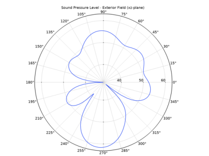
Locate the Title section. In the Title text area, type Sound Pressure Level - Exterior Field (xz-plane).
|
|
1
|
|
2
|
|
3
|
|
4
|
|
5
|
|
6
|
|
1
|
|
2
|
|
3
|
|
4
|
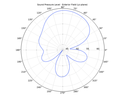
Locate the Title section. In the Title text area, type Sound Pressure Level - Exterior Field (yz-plane).
|
|
1
|
|
2
|
|
3
|
|
4
|
|
5
|
|
6
|
|
1
|
|
2
|
|
3
|
|
4
|
|
5
|
|
1
|
|
2
|
|
3
|
|
4
|
|
5
|
|
6
|
|
7
|
|
8
|
|
9
|
|
10
|
|
1
|
|
2
|
|
3
|
|
4
|
|
5
|
|
1
|
|
2
|
|
3
|
|
4
|
|
5
|
|
6
|
|
7
|
|
8
|
|
1
|
|
2
|
|
3
|
|
4
|
|
5
|
|
6
|
|
7
|
|
8
|
|
1
|
|
2
|
|
3
|
|
4
|
|
1
|
|
2
|
|
3
|
|
4
|
|
1
|
|
2
|
|
3
|
|
4
|
|
5
|
|
6
|
|
1
|
|
2
|
|
3
|
|
1
|
|
2
|
|
3
|
|
4
|
|
1
|
|
2
|
|
3
|
|
1
|
|
2
|