|
|
|


|
•
|
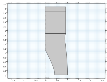
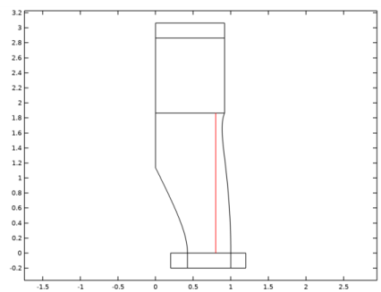
A cylindrical domain — adjoined at the inlet plane and extending to the terminal plane, z = 2.86393 — extends the modeling domain into a region where you can consider the mean flow as being uniform. This allows you to impose the simple boundary condition of a constant velocity potential and a vanishing tangential velocity for the background flow at the terminal plane.
|
|
•
|
Sound hard — the normal component of the acoustic particle velocity vanishes at the boundary.
|
|
•
|
Impedance — the normal component of the acoustic particle velocity is related to the particle displacement through the equation
|
|
•
|
Compressible Potential Flow (cpf) — for modeling the background mean-flow velocity field as a potential flow (a lossless and irrotational flow).
|
|
•
|
Linearized Potential Flow, Boundary Mode (aebm) — for calculating the boundary eigenmode to be used as the source of the acoustic noise in the background mean-flow.
|
|
•
|
Linearized Potential Flow, Frequency Domain (ae, ae2) — for modeling the time-harmonic acoustic field above and below the source plane.
|
|
1
|
|
2
|
|
3
|
Click Add.
|
|
4
|
In the Select Physics tree, select Acoustics>Aeroacoustics>Linearized Potential Flow, Boundary Mode (aebm).
|
|
5
|
Click Add.
|
|
6
|
|
7
|
In the Select Physics tree, select Acoustics>Aeroacoustics>Linearized Potential Flow, Frequency Domain (ae).
|
|
8
|
Click Add twice.
|
|
9
|
Click
|
|
10
|
|
11
|
Click
|
|
1
|
|
2
|
|
3
|
|
1
|
|
2
|
|
3
|
|
4
|
Browse to the model’s Application Libraries folder and double-click the file flow_duct_parameters.txt.
|
|
1
|
|
2
|
|
3
|
Click
|
|
4
|
|
5
|
Click
|
|
1
|
|
2
|
|
3
|
|
4
|
|
5
|
|
6
|
|
7
|
|
9
|
|
10
|
|
1
|
|
2
|
|
3
|
|
4
|
|
5
|
|
6
|
|
7
|
|
1
|
|
2
|
|
3
|
|
4
|
On the object imp1, select Boundary 34 only.
|
|
5
|
|
6
|
|
7
|
|
8
|
|
1
|
|
2
|
|
1
|
|
3
|
|
4
|
|
1
|
|
3
|
|
4
|
|
1
|
|
3
|
|
4
|
|
1
|
|
3
|
|
4
|
|
1
|
|
3
|
|
4
|
|
1
|
|
3
|
|
4
|
|
1
|
|
1
|
|
3
|
|
4
|
|
5
|
|
1
|
|
2
|
|
3
|
|
5
|
Locate the Variables section. In the table, enter the following settings:
|
|
1
|
|
2
|
|
3
|
|
5
|
Locate the Variables section. In the table, enter the following settings:
|
|
1
|
|
2
|
|
3
|
|
1
|
|
2
|
|
3
|
|
1
|
|
2
|
|
1
|
|
2
|
|
3
|
|
4
|
|
5
|
|
1
|
|
3
|
|
4
|
|
5
|
|
6
|
|
1
|
In the Model Builder window, under Component 1 (comp1)>Compressible Potential Flow (cpf) click Compressible Potential Flow Model 1.
|
|
2
|
In the Settings window for Compressible Potential Flow Model, locate the Compressible Potential Flow Model section.
|
|
3
|
|
1
|
|
1
|
|
1
|
In the Model Builder window, under Component 1 (comp1) click Linearized Potential Flow, Boundary Mode (aebm).
|
|
2
|
In the Settings window for Linearized Potential Flow, Boundary Mode, locate the Boundary Selection section.
|
|
3
|
|
5
|
|
1
|
In the Model Builder window, under Component 1 (comp1)>Linearized Potential Flow, Boundary Mode (aebm) click Linearized Potential Flow Model 1.
|
|
2
|
In the Settings window for Linearized Potential Flow Model, locate the Linearized Potential Flow Model section.
|
|
3
|
|
4
|
|
5
|
Specify the V vector as
|
|
6
|
|
1
|
|
2
|
|
1
|
|
2
|
|
3
|
|
4
|
|
5
|
|
7
|
|
1
|
|
2
|
|
3
|
Click
|
|
5
|
|
1
|
|
2
|
|
3
|
Locate the Data section. From the Dataset list, choose Study 1 - Background and Source/Parametric Solutions 1 (sol3).
|
|
1
|
|
2
|
|
3
|
|
1
|
|
2
|
|
1
|
|
2
|
|
3
|
|
4
|
|
5
|
Locate the Data section. From the Dataset list, choose Study 1 - Background and Source/Parametric Solutions 1 (sol3).
|
|
6
|
Click
|
|
7
|
|
1
|
|
2
|
|
3
|
|
4
|
|
5
|
|
6
|
|
7
|
|
1
|
|
2
|
|
3
|
|
4
|
|
5
|
|
6
|
|
7
|
|
1
|
|
2
|
|
3
|
|
4
|
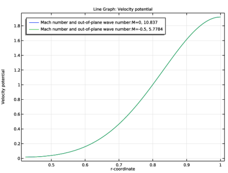
Locate the Legends section. In the table, enter the following settings:
|
|
5
|
|
1
|
|
2
|
In the Settings window for 1D Plot Group, type Boundary Mode Potential: phi_b in the Label text field.
|
|
3
|
Locate the Data section. From the Dataset list, choose Study 1 - Background and Source/Parametric Solutions 1 (sol3).
|
|
4
|
|
5
|
|
1
|
|
2
|
|
3
|
|
5
|
|
6
|
|
7
|
Find the Prefix and suffix subsection. In the Prefix text field, type Mach number and out-of-plane wave number: .
|
|
8
|
|
9
|
|
10
|
|
1
|
|
1
|
|
2
|
|
1
|
|
3
|
|
4
|
|
5
|
|
6
|
|
1
|
|
2
|
|
3
|
|
5
|
|
1
|
In the Model Builder window, under Component 1 (comp1) click Linearized Potential Flow, Frequency Domain (ae).
|
|
3
|
In the Settings window for Linearized Potential Flow, Frequency Domain, click to expand the Equation section.
|
|
4
|
|
1
|
|
3
|
|
4
|
|
1
|
|
3
|
|
4
|
|
1
|
|
3
|
|
4
|
|
1
|
In the Model Builder window, under Component 1 (comp1) click Linearized Potential Flow, Frequency Domain 2 (ae2).
|
|
3
|
In the Settings window for Linearized Potential Flow, Frequency Domain, locate the Linearized Potential Flow Equation Settings section.
|
|
4
|
|
1
|
In the Model Builder window, under Component 1 (comp1)>Linearized Potential Flow, Frequency Domain 2 (ae2) click Linearized Potential Flow Model 1.
|
|
2
|
In the Settings window for Linearized Potential Flow Model, locate the Linearized Potential Flow Model section.
|
|
3
|
|
4
|
|
5
|
Specify the V vector as
|
|
1
|
Right-click Component 1 (comp1)>Linearized Potential Flow, Frequency Domain 2 (ae2)>Linearized Potential Flow Model 1 and choose Duplicate.
|
|
3
|
In the Settings window for Linearized Potential Flow Model, locate the Linearized Potential Flow Model section.
|
|
4
|
Specify the V vector as
|
|
1
|
|
3
|
|
4
|
|
1
|
|
2
|
|
3
|
Find the Physics interfaces in study subsection. In the table, clear the Solve check boxes for Compressible Potential Flow (cpf) and Linearized Potential Flow, Boundary Mode (aebm).
|
|
4
|
|
5
|
|
6
|
|
7
|
Find the Physics interfaces in study subsection. In the table, clear the Solve check boxes for Compressible Potential Flow (cpf) and Linearized Potential Flow, Boundary Mode (aebm).
|
|
8
|
|
9
|
Find the Studies subsection. In the Select Study tree, select Preset Studies for Some Physics Interfaces>Frequency Domain.
|
|
10
|
Find the Physics interfaces in study subsection. In the table, clear the Solve check boxes for Compressible Potential Flow (cpf) and Linearized Potential Flow, Boundary Mode (aebm).
|
|
11
|
|
12
|
Find the Studies subsection. In the Select Study tree, select Preset Studies for Some Physics Interfaces>Frequency Domain.
|
|
13
|
Find the Physics interfaces in study subsection. In the table, clear the Solve check boxes for Compressible Potential Flow (cpf) and Linearized Potential Flow, Boundary Mode (aebm).
|
|
14
|
|
15
|
|
1
|
|
2
|
|
3
|
|
4
|
|
1
|
In the Model Builder window, under Study 2 - Frequency Domain (M = 0, lined) click Step 1: Frequency Domain.
|
|
2
|
|
3
|
|
4
|
Click to expand the Values of Dependent Variables section. Find the Values of variables not solved for subsection. From the Settings list, choose User controlled.
|
|
5
|
|
6
|
|
7
|
|
8
|
|
9
|
|
1
|
|
2
|
|
3
|
|
4
|
|
1
|
In the Model Builder window, under Study 3 - Frequency Domain (M = -0.5, lined) click Step 1: Frequency Domain.
|
|
2
|
|
3
|
|
4
|
Locate the Values of Dependent Variables section. Find the Values of variables not solved for subsection. From the Settings list, choose User controlled.
|
|
5
|
|
6
|
|
7
|
|
8
|
|
9
|
|
1
|
|
2
|
|
3
|
|
4
|
|
1
|
In the Model Builder window, under Study 4 - Frequency Domain (M = 0, hard wall) click Step 1: Frequency Domain.
|
|
2
|
|
3
|
|
4
|
Locate the Physics and Variables Selection section. Select the Modify model configuration for study step check box.
|
|
5
|
In the tree, select Component 1 (Comp1)>Linearized Potential Flow, Frequency Domain (Ae)>Impedance 1.
|
|
6
|
Click
|
|
7
|
In the tree, select Component 1 (Comp1)>Linearized Potential Flow, Frequency Domain (Ae)>Impedance 2.
|
|
8
|
Click
|
|
9
|
Locate the Values of Dependent Variables section. Find the Values of variables not solved for subsection. From the Settings list, choose User controlled.
|
|
10
|
|
11
|
|
12
|
|
13
|
|
14
|
|
1
|
|
2
|
|
3
|
|
4
|
|
1
|
In the Model Builder window, under Study 5 - Frequency Domain (M = -0.5, hard wall) click Step 1: Frequency Domain.
|
|
2
|
|
3
|
|
4
|
Locate the Physics and Variables Selection section. Select the Modify model configuration for study step check box.
|
|
5
|
In the tree, select Component 1 (Comp1)>Linearized Potential Flow, Frequency Domain (Ae)>Impedance 1.
|
|
6
|
Click
|
|
7
|
In the tree, select Component 1 (Comp1)>Linearized Potential Flow, Frequency Domain (Ae)>Impedance 2.
|
|
8
|
Click
|
|
9
|
Locate the Values of Dependent Variables section. Find the Values of variables not solved for subsection. From the Settings list, choose User controlled.
|
|
10
|
|
11
|
|
12
|
|
13
|
|
14
|
|
1
|
|
2
|
|
3
|
|
4
|
|
1
|
|
2
|
|
3
|
|
4
|
|
5
|
|
6
|
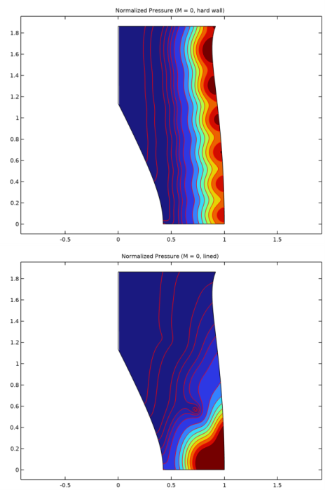
Locate the Data section. From the Dataset list, choose Study 2 - Frequency Domain (M = 0, lined)/Solution 6 (sol6).
|
|
1
|
|
2
|
|
3
|
|
4
|
|
5
|
In the Levels text field, type 0.0001 0.001 0.01 0.02 0.04 0.06 0.1 0.2 0.3 0.4 0.5 0.6 0.7 0.8 0.9.
|
|
6
|
|
7
|
|
8
|
|
1
|
|
2
|
|
3
|
|
4
|
|
5
|
In the Levels text field, type 0.0001 0.001 0.01 0.02 0.04 0.06 0.1 0.2 0.3 0.4 0.5 0.6 0.7 0.8 0.9.
|
|
6
|
|
7
|
|
8
|
|
1
|
|
2
|
|
3
|
|
1
|
|
2
|
|
3
|
|
1
|
|
2
|
|
3
|
|
1
|
|
2
|
|
3
|
|
1
|
|
2
|
|
3
|
|
1
|
|
2
|
|
3
|
|
4
|
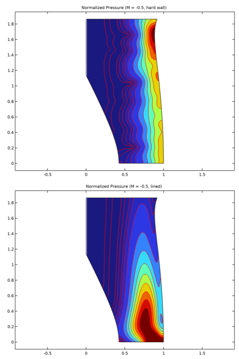
Locate the Data section. From the Dataset list, choose Study 3 - Frequency Domain (M = -0.5, lined)/Solution 7 (sol7).
|
|
5
|
|
6
|
|
1
|
|
2
|
|
3
|
|
4
|
Locate the Data section. From the Dataset list, choose Study 4 - Frequency Domain (M = 0, hard wall)/Solution 8 (sol8).
|
|
5
|
|
6
|
|
1
|
|
2
|
In the Settings window for 2D Plot Group, type Pressure: M = -0.5, hard wall in the Label text field.
|
|
3
|
|
4
|
Locate the Data section. From the Dataset list, choose Study 5 - Frequency Domain (M = -0.5, hard wall)/Solution 9 (sol9).
|
|
5
|
|
6
|
|
1
|
|
2
|
In the Settings window for Global Evaluation, type Global Evaluation: W_src (M = 0) in the Label text field.
|
|
3
|
Locate the Data section. From the Dataset list, choose Study 1 - Background and Source/Parametric Solutions 1 (sol3).
|
|
4
|
|
5
|
|
6
|
Locate the Expressions section. In the table, enter the following settings:
|
|
7
|
Click
|
|
1
|
|
2
|
In the Settings window for Global Evaluation, type Global Evaluation: W_src (M = -0.5) in the Label text field.
|
|
3
|
|
4
|
|
1
|
|
2
|
In the Settings window for Global Evaluation, type Global Evaluation: W_inl (M = 0, lined) in the Label text field.
|
|
3
|
Locate the Data section. From the Dataset list, choose Study 2 - Frequency Domain (M = 0, lined)/Solution 6 (sol6).
|
|
4
|
Locate the Expressions section. In the table, enter the following settings:
|
|
5
|
|
1
|
|
2
|
In the Settings window for Global Evaluation, type Global Evaluation: W_inl (M = -0.5, lined) in the Label text field.
|
|
3
|
Locate the Data section. From the Dataset list, choose Study 3 - Frequency Domain (M = -0.5, lined)/Solution 7 (sol7).
|
|
4
|
|
1
|
|
2
|
In the Settings window for Global Evaluation, type Global Evaluation: Attenuation (M = 0, lined) in the Label text field.
|
|
3
|
Locate the Data section. From the Dataset list, choose Study 2 - Frequency Domain (M = 0, lined)/Solution 6 (sol6).
|
|
4
|
Locate the Expressions section. In the table, enter the following settings:
|
|
5
|
Click
|
|
1
|
|
2
|
In the Settings window for Global Evaluation, type Global Evaluation: Attenuation (M = -0.5, lined) in the Label text field.
|
|
3
|
Locate the Expressions section. In the table, enter the following settings:
|
|
4
|