|
|
|

|
1
|
|
2
|
In the Select Physics tree, select Acoustics>Pressure Acoustics>Pressure Acoustics, Frequency Domain (acpr).
|
|
3
|
Click Add.
|
|
4
|
In the Select Physics tree, select Acoustics>Pressure Acoustics>Pressure Acoustics, Boundary Elements (pabe).
|
|
5
|
Click Add.
|
|
6
|
Click
|
|
7
|
|
8
|
Click
|
|
1
|
|
2
|
|
3
|
|
4
|
|
5
|
|
6
|
|
7
|
|
1
|
|
2
|
|
3
|
|
4
|
|
5
|
|
1
|
|
2
|
|
3
|
Select the object pt1 only.
|
|
4
|
|
5
|
|
6
|
|
7
|
|
8
|
|
9
|
Locate the Selections of Resulting Entities section. Select the Resulting objects selection check box.
|
|
10
|
|
11
|
|
1
|
|
2
|
|
1
|
|
2
|
|
4
|
|
5
|
|
6
|
|
7
|
Click OK.
|
|
1
|
|
2
|
|
4
|
|
5
|
|
6
|
|
7
|
Click OK.
|
|
1
|
|
2
|
|
4
|
|
5
|
|
6
|
|
7
|
Click OK.
|
|
1
|
|
2
|
|
4
|
|
5
|
|
6
|
|
7
|
Click OK.
|
|
1
|
|
2
|
|
4
|
|
5
|
|
6
|
|
7
|
Click OK.
|
|
1
|
|
2
|
|
3
|
In the tree, select Built-in>Air.
|
|
4
|
|
5
|
|
1
|
|
2
|
|
1
|
In the Model Builder window, under Component 1 (comp1) right-click Pressure Acoustics, Frequency Domain (acpr) and choose Points>Monopole Point Source.
|
|
2
|
|
3
|
|
4
|
|
1
|
In the Model Builder window, under Component 1 (comp1) click Pressure Acoustics, Boundary Elements (pabe).
|
|
2
|
In the Settings window for Pressure Acoustics, Boundary Elements, locate the Domain Selection section.
|
|
3
|
|
1
|
|
2
|
|
3
|
|
1
|
|
2
|
|
3
|
|
4
|
|
1
|
|
2
|
|
1
|
|
2
|
|
3
|
|
1
|
|
2
|
|
3
|
|
4
|
Locate the Pressure Acoustics, Frequency Domain (acpr) section. From the Number of mesh elements per wavelength list, choose User defined.
|
|
6
|
|
7
|
|
1
|
|
2
|
|
3
|
|
4
|
|
5
|
|
6
|
|
7
|
|
8
|
|
9
|
|
10
|
|
1
|
|
2
|
|
3
|
|
4
|
|
5
|
|
6
|
|
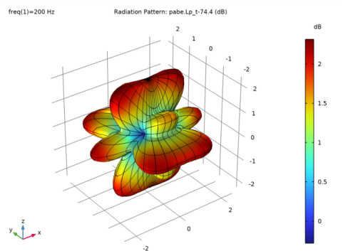
1
|
In the Model Builder window, under Results>Acoustic Pressure (pabe) right-click Multislice 1 and choose Duplicate.
|
|
2
|
|
3
|
|
4
|
|
5
|
|
6
|
|
7
|
|
8
|
|
1
|
|
1
|
|
2
|
|
3
|
|
1
|
|
2
|
|
3
|
|
4
|
Locate the Evaluation section. Find the Angles subsection. In the Number of elevation angles text field, type 50.
|
|
5
|
|
6
|
|
7
|
|
8
|
|
9
|
|
10
|
|
1
|
|
2
|
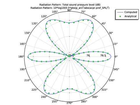
In the Settings window for Polar Plot Group, type Spatial Response in xz-plane in the Label text field.
|
|
1
|
|
2
|
|
3
|
|
4
|
Locate the Evaluation section. Find the Angles subsection. In the Number of angles text field, type 360.
|
|
5
|
|
6
|
|
7
|
|
8
|
|
9
|
|
1
|
|
2
|
|
3
|
|
4
|
Click to expand the Coloring and Style section. Find the Line style subsection. From the Line list, choose None.
|
|
5
|
|
6
|
|
7
|
Locate the Legends section. In the table, enter the following settings:
|
|
8
|