PDF

Quadrupole Lens
Introduction
Just like optical lenses focus light, electric and magnetic lenses can focus beams of charged particles. Systems of magnetic quadrupole lenses find a common use in focusing both ion and particle beams in accelerators at nuclear and particle physics centers such as CERN, SLAC, and ISIS. This COMSOL Multiphysics model shows the path of B5+ ions going through three consecutive magnetic quadrupole lenses. This 3D model takes fringing fields into account, and the calculation of the forces on the ions uses all components of their velocities.
Model Definition
The quadrupole consists of an assembly of four permanent magnets, as seen in Figure 1, where the magnets work together to give a good approximation of a quadrupole field. To strengthen the field and keep it contained within the system, the magnets are set in an iron cylinder.
Figure 1: Cross-sectional view of one of the magnetic quadrupoles used in the lens. The arrows show the direction of the magnetization.
The ions are sent through a system of three consecutive quadrupole assemblies. The middle one is twice as long as the other ones, and is rotated by 90 degrees around the central axis. This means the polarity of its magnets is reversed. Figure 2 gives a full view of the magnetic quadrupole lens.
Figure 2: Cutout of the quadrupole lens. The second quadrupole (Q2) has its polarities reversed compared to Q1 and Q3. After traveling through the lens, the ions are left to drift 1 m.
An accelerator feeds the system with ions traveling with the velocity 0.01c along the central axis. To study the focusing effect of the quadrupoles, track a number of ions starting out from a distance of 3 cm from the central axis, evenly distributed along the circumference of a circle in the transverse plane. They are all assumed to have a zero initial transverse velocity. Each quadrupole focuses the ion beam along one of the transverse axes and defocuses it along the other one. The net effect after traveling through the system of the three quadrupoles and the drift length is focusing in all directions. As the ions exit the system, they are all contained within a 1 cm radius in the transverse plane.
The geometry of the quadrupole lens is composed of three quadrupoles in a row, followed by 1 m of empty space, where the ions are left to drift. The AC/DC Module features a physics interface for magnetostatics in absence of currents. The formulation used in this physics interface reduces the memory usage considerably compared to the formulation including currents.
Domain Equations
The magnetic field is described using a static magnetic equation solving for the magnetic scalar potential Vm (Wb/m):
where μ0 = 4π·107 H/m denotes the permeability of vacuum and M is the magnetization (A/m). In the iron domain
where μr = 4000 is the relative permeability. The magnetic scalar potential is everywhere defined so that H = ∇Vm. 
Boundary Conditions
The magnetic insulation boundary condition, reading n·B = 0, is used all around the iron cylinder, and at the lateral surfaces of the air domain that encloses the drift length.
Results
The x-component of the magnetic field density and arrows showing its local direction are shown in the figure below.
Figure 3: Arrows of the magnetic field and slices of its x-component in the quadrupole lens.
Each ion passing through the assembly experiences Maxwell forces equal to F = qv × B, where v (SI unit: m/s) is the velocity of the ion. To find the transverse position as a function of time, solve Newton’s second law for each ion: qv × B = ma. This particle tracing operation can be performed in postprocessing (in a Plot Group) and does not require the Particle Tracing Module. Figure 4 shows the traces of the ions as they fly through the quadrupole lens.
Figure 4: Particle tracing plots of the ions. Two cross-sections of the geometry are shown. The line colors show the local force acting on each ion. The force grows larger (red) far away from the center of the beam line and smaller (blue) where two oppositely polarized quadrupoles join. The z-axis is rescaled in the top figure.
Application Library path: ACDC_Module/Other_Industrial_Applications/quadrupole_lens
Modeling Instructions
From the File menu, choose New.
New
In the New window, click  Model Wizard.
Model Wizard
1
In the Model Wizard window, click  3D.
2
In the Select Physics tree, select AC/DC>Magnetic Fields, No Currents>Magnetic Fields, No Currents (mfnc).
3
Click Add.
4
Click  Study.
5
In the Select Study tree, select General Studies>Stationary.
6
Geometry 1
Import 1 (imp1)
1
In the Home toolbar, click  Import.
2
In the Settings window for Import, locate the Import section.
3
Click  Browse.
4
5
Click  Import.
Global Definitions
Parameters 1
1
In the Model Builder window, under Global Definitions click Parameters 1.
2
In the Settings window for Parameters, locate the Parameters section.
3
Click  Load from File.
4
Create a rotated coordinate system to simplify the definition of the magnetization in the magnets.
Definitions
Rotated System 2 (sys2)
1
In the Definitions toolbar, click  Coordinate Systems and choose Rotated System.
2
In the Settings window for Rotated System, locate the Rotation section.
3
Find the Euler angles (Z-X-Z) subsection. In the γ text field, type pi/4.
Materials
Iron
1
In the Model Builder window, under Component 1 (comp1) right-click Materials and choose Blank Material.
2
Right-click Material 1 (mat1) and choose Rename.
3
In the Rename Material dialog box, type Iron in the New label text field.
4
5
6
In the Settings window for Material, locate the Material Contents section.
7
Air
1
In the Model Builder window, right-click Materials and choose Blank Material.
2
Right-click Material 2 (mat2) and choose Rename.
3
In the Rename Material dialog box, type Air in the New label text field.
4
5
6
In the Settings window for Material, locate the Material Contents section.
7
Magnetic Fields, No Currents (mfnc)
Magnetic Flux Conservation 2
1
In the Model Builder window, under Component 1 (comp1) right-click Magnetic Fields, No Currents (mfnc) and choose Magnetic Flux Conservation.
2
3
In the Settings window for Magnetic Flux Conservation, locate the Coordinate System Selection section.
4
From the Coordinate system list, choose Rotated System 2 (sys2).
5
Locate the Constitutive Relation B-H section. From the Magnetization model list, choose Magnetization.
6
Specify the M vector as
Magnetic Flux Conservation 3
1
In the Physics toolbar, click  Domains and choose Magnetic Flux Conservation.
2
3
In the Settings window for Magnetic Flux Conservation, locate the Coordinate System Selection section.
4
From the Coordinate system list, choose Rotated System 2 (sys2).
5
Locate the Constitutive Relation B-H section. From the Magnetization model list, choose Magnetization.
6
Specify the M vector as
Magnetic Flux Conservation 4
1
In the Physics toolbar, click  Domains and choose Magnetic Flux Conservation.
2
3
In the Settings window for Magnetic Flux Conservation, locate the Coordinate System Selection section.
4
From the Coordinate system list, choose Rotated System 2 (sys2).
5
Locate the Constitutive Relation B-H section. From the Magnetization model list, choose Magnetization.
6
Specify the M vector as
Magnetic Flux Conservation 5
1
In the Physics toolbar, click  Domains and choose Magnetic Flux Conservation.
2
3
In the Settings window for Magnetic Flux Conservation, locate the Coordinate System Selection section.
4
From the Coordinate system list, choose Rotated System 2 (sys2).
5
Locate the Constitutive Relation B-H section. From the Magnetization model list, choose Magnetization.
6
Specify the M vector as
Add a zero potential point condition to fix the magnetic scalar potential. Without it, the solution would be determined only up to a constant.
Zero Magnetic Scalar Potential 1
1
In the Physics toolbar, click  Points and choose Zero Magnetic Scalar Potential.
2
Mesh 1
1
In the Model Builder window, under Component 1 (comp1) click Mesh 1.
2
In the Settings window for Mesh, locate the Physics-Controlled Mesh section.
3
From the Element size list, choose Fine.
4
Click  Build All.
Study 1
1
In the Model Builder window, click Study 1.
2
In the Settings window for Study, locate the Study Settings section.
3
Clear the Generate default plots check box.
4
In the Home toolbar, click  Compute.
Results
Magnetic Field
1
In the Home toolbar, click  Add Plot Group and choose 3D Plot Group.
2
In the Settings window for 3D Plot Group, type Magnetic Field in the Label text field.
Slice 1
1
Right-click Magnetic Field and choose Slice.
2
In the Settings window for Slice, locate the Plane Data section.
3
In the Planes text field, type 1.
4
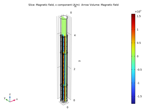
Click Replace Expression in the upper-right corner of the Expression section. From the menu, choose Component 1 (comp1)>Magnetic Fields, No Currents>Magnetic>Magnetic field - A/m>mfnc.Hx - Magnetic field, x component.
5
In the Magnetic Field toolbar, click  Plot.
The plot now shows the x-component of the magnetic field.
Arrow Volume 1
1
In the Model Builder window, right-click Magnetic Field and choose Arrow Volume.
2
In the Settings window for Arrow Volume, click Replace Expression in the upper-right corner of the Expression section. From the menu, choose Component 1 (comp1)>Magnetic Fields, No Currents>Magnetic>mfnc.Hx,mfnc.Hy,mfnc.Hz - Magnetic field.
3
Locate the Arrow Positioning section. Find the x grid points subsection. In the Points text field, type 4.
4
Find the y grid points subsection. In the Points text field, type 4.
5
Find the z grid points subsection. In the Points text field, type 20.
6
Locate the Coloring and Style section. From the Color list, choose Black.
7
In the Magnetic Field toolbar, click  Plot.
Add a new plot group to trace the ions as they travel through the system of quadrupoles.
Ion Tracing
1
In the Home toolbar, click  Add Plot Group and choose 3D Plot Group.
2
Click the  Show More Options button in the Model Builder toolbar.
3
In the Show More Options dialog box, in the tree, select the check box for the node Results>All Plot Types.
4
5
In the Settings window for 3D Plot Group, type Ion Tracing in the Label text field.
Particle Tracing with Mass 1
1
In the Ion Tracing toolbar, click  More Plots and choose Particle Tracing with Mass.
The default expression for the force is the magnetic force acting on the ions. Enter the values of the paramters.
2
In the Settings window for Particle Tracing with Mass, locate the Total Force section.
3
Find the Parameters subsection. In the table, enter the following settings:
4
Click to expand the Mass and Velocity section. In the Mass text field, type m.
5
Find the Initial velocity subsection. In the z component text field, type vz.
6
Locate the Particle Positioning section. In the x text field, type 0.03*cos(range(0,0.05*pi,2*pi)).
7
In the y text field, type 0.03*sin(range(0,0.05*pi,2*pi)).
8
In the z text field, type 0.01.
9
Click to expand the Coloring and Style section. Find the Line style subsection. From the Type list, choose Tube.
10
Select the Radius scale factor check box.
11
In the Tube radius expression text field, type 0.001.
12
Click to expand the Quality section. Find the ODE solver settings subsection. In the Relative tolerance text field, type 1e-6.
13
In the Ion Tracing toolbar, click  Plot.
Color the traces using the magnitude of the local force acting on each ion.
Color Expression 1
1
Right-click Particle Tracing with Mass 1 and choose Color Expression.
2
In the Settings window for Color Expression, locate the Expression section.
3
In the Expression text field, type q*vz*mfnc.normB.
4
In the Ion Tracing toolbar, click  Plot.
Create a new View with a rescaled geometry to better visualize the trajectory of the ions.
Definitions
Default View
1
In the Model Builder window, under Component 1 (comp1)>Definitions click View 1.
2
In the Settings window for View, type Default View in the Label text field.
Scaled View
1
In the Definitions toolbar, click  View.
2
In the Settings window for View, type Scaled View in the Label text field.
Camera
1
In the Model Builder window, expand the Scaled View node, then click Camera.
2
In the Settings window for Camera, locate the Camera section.
3
From the View scale list, choose Automatic.
Use the new View in the tracing plot.
Results
Ion Tracing
1
In the Model Builder window, under Results click Ion Tracing.
2
In the Settings window for 3D Plot Group, locate the Plot Settings section.
3
From the View list, choose Scaled View.
4
In the Ion Tracing toolbar, click  Plot.
5
Use the Go to XY View and Zoom buttons to reproduce the plots in Figure 4.
Finally, specify that magnetic field plot must use the default view.
Magnetic Field
1
In the Model Builder window, click Magnetic Field.
2
In the Settings window for 3D Plot Group, locate the Plot Settings section.
3
From the View list, choose Default View.
4
In the Magnetic Field toolbar, click  Plot.