|
|
|
|
1
|
|
2
|
In the Select Physics tree, select AC/DC>Electromagnetics and Mechanics>Rotating Machinery, Magnetic (rmm).
|
|
3
|
Click Add.
|
|
4
|
Click
|
|
5
|
|
6
|
Click
|
|
1
|
|
2
|
|
1
|
|
2
|
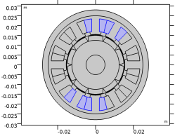
In the Part Libraries window, select AC/DC Module>Rotating Machinery 2D>Rotors>Internal>surface_mounted_magnet_internal_rotor_2d in the tree.
|
|
3
|
|
1
|
In the Model Builder window, under Component 1 (comp1)>Geometry 1 click Internal Rotor – Surface Mounted Magnets 1 (pi1).
|
|
2
|
|
4
|
|
1
|
|
2
|
|
3
|
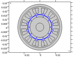
In the Part Libraries window, select AC/DC Module>Rotating Machinery 2D>Stators>External>slotted_external_stator_2d in the tree.
|
|
4
|
|
1
|
In the Model Builder window, under Component 1 (comp1)>Geometry 1 click External Stator – Slotted 1 (pi2).
|
|
2
|
|
4
|
|
1
|
|
2
|
|
3
|
|
4
|
|
5
|
|
1
|
|
2
|
|
3
|
|
4
|
Locate the Variables section. In the table, enter the following settings:
|
|
1
|
|
2
|
|
3
|
|
4
|
|
5
|
|
6
|
|
1
|
|
2
|
|
3
|
Locate the Variables section. In the table, enter the following settings:
|
|
1
|
|
2
|
|
3
|
|
4
|
In the Add dialog box, in the Selections to add list, choose Rotor air (Internal Rotor – Surface Mounted Magnets 1) and Stator air (External Stator – Slotted 1).
|
|
5
|
|
1
|
|
2
|
|
3
|
|
4
|
In the Add dialog box, in the Selections to add list, choose Rotor iron (Internal Rotor – Surface Mounted Magnets 1) and Stator iron (External Stator – Slotted 1).
|
|
5
|
|
1
|
|
2
|
|
3
|
In the tree, select Built-in>Air.
|
|
4
|
|
5
|
|
6
|
|
7
|
In the tree, select AC/DC>Copper.
|
|
8
|
|
9
|
In the tree, select AC/DC>Hard Magnetic Materials>Sintered NdFeB Grades (Chinese Standard)>N54 (Sintered NdFeB).
|
|
10
|
|
11
|
In the tree, select Built-in>Iron.
|
|
12
|
|
13
|
|
1
|
In the Model Builder window, under Component 1 (comp1)>Materials click Soft Iron (Without Losses) (mat2).
|
|
2
|
|
3
|
|
1
|
|
2
|
|
3
|
|
4
|
|
1
|
|
2
|
|
3
|
|
1
|
|
2
|
|
3
|
|
1
|
|
2
|
|
3
|
|
1
|
|
2
|
|
3
|
|
1
|
|
2
|
|
3
|
|
4
|
|
1
|
|
2
|
|
3
|
|
1
|
|
2
|
|
3
|
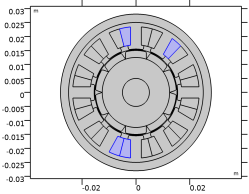
Locate the Domain Selection section. From the Selection list, choose Odd magnets (Internal Rotor – Surface Mounted Magnets 1).
|
|
4
|
Locate the Coordinate System Selection section. From the Coordinate system list, choose Cylindrical System 2 (sys2).
|
|
5
|
Locate the Constitutive Relation B-H section. From the Magnetization model list, choose Remanent flux density.
|
|
6
|
|
1
|
|
2
|
|
3
|
Locate the Domain Selection section. From the Selection list, choose Even magnets (Internal Rotor – Surface Mounted Magnets 1).
|
|
4
|
|
1
|
|
2
|
|
3
|
|
4
|
|
5
|
Click OK.
|
|
6
|
|
7
|
|
8
|
|
9
|
|
10
|
|
11
|
|
1
|
|
2
|
|
3
|
|
4
|
|
5
|
|
1
|
|
2
|
|
3
|
|
4
|
|
5
|
|
6
|
Click OK.
|
|
7
|
|
8
|
|
1
|
|
2
|
|
3
|
|
4
|
|
5
|
|
6
|
Click OK.
|
|
1
|
|
2
|
|
3
|
|
4
|
|
5
|
|
6
|
Click OK.
|
|
7
|
|
8
|
|
1
|
|
2
|
|
3
|
|
4
|
|
5
|
|
6
|
Click OK.
|
|
1
|
|
2
|
|
3
|
|
4
|
Click the Custom button.
|
|
5
|
|
6
|
|
7
|
|
1
|
|
2
|
In the Settings window for Study, type Study 1: Initial angle parametric sweep at DC current in the Label text field.
|
|
1
|
In the Model Builder window, under Study 1: Initial angle parametric sweep at DC current click Step 1: Stationary.
|
|
2
|
|
3
|
Select the Plot check box.
|
|
4
|
|
5
|
Click
|
|
7
|
|
1
|
|
2
|
|
1
|
|
2
|
|
3
|
|
4
|
|
5
|
|
1
|
|
2
|
|
3
|
|
4
|
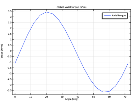
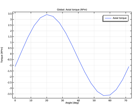
In the associated text field, type Angle [deg].
|
|
5
|
|
6
|
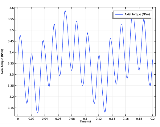
In the associated text field, type Torque [N*m].
|
|
1
|
|
2
|
|
4
|
|
1
|
|
2
|
|
1
|
|
2
|
|
3
|
|
4
|
Select the Description check box.
|
|
1
|
|
2
|
|
3
|
|
4
|
|
5
|
|
1
|
|
2
|
|
1
|
|
2
|
|
3
|
|
1
|
|
2
|
|
3
|
In the Model Builder window, expand the Study 2: Synchronous rotation>Solver Configurations>Solution 2 (sol2)>Time-Dependent Solver 1 node, then click Fully Coupled 1.
|
|
4
|
|
5
|
|
1
|
|
2
|
In the Settings window for Rotating Machinery, Magnetic, click to expand the Discretization section.
|
|
3
|
|
4
|
|
1
|
|
2
|
|
1
|
In the Model Builder window, under Component 1 (comp1)>Geometry 1 click Internal Rotor – Surface Mounted Magnets 1 (pi1).
|
|
2
|
|
4
|
|
1
|
|
2
|
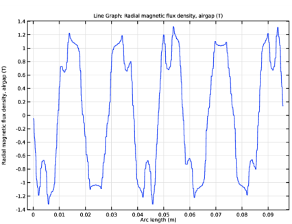
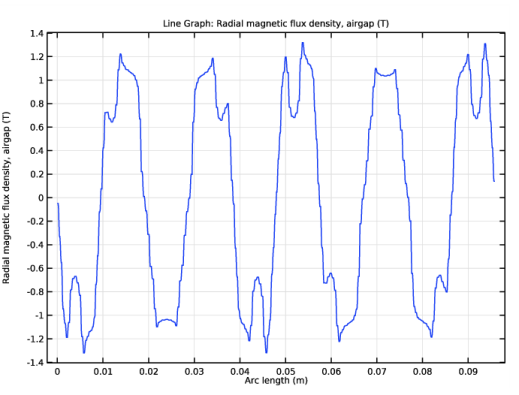
In the Settings window for 1D Plot Group, type Air Gap Radial Magnetic Flux Density in the Label text field.
|
|
3
|
Locate the Data section. From the Dataset list, choose Study 2: Synchronous rotation/Solution 2 (sol2).
|
|
4
|
|
1
|
|
2
|
|
3
|
|
4
|
|
5
|
|
1
|
|
2
|
|
3
|
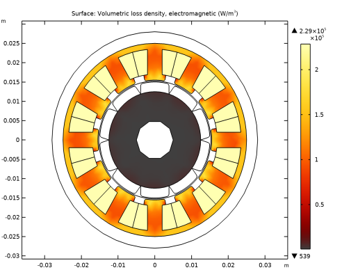
Find the Studies subsection. In the Select Study tree, select Preset Studies for Selected Physics Interfaces>Time to Frequency Losses.
|
|
4
|
|
5
|
|
1
|
|
2
|
In the Settings window for Study, type Study 3: Loss calculation over full rotation in the Label text field.
|
|
1
|
In the Model Builder window, under Study 3: Loss calculation over full rotation click Step 1: Time to Frequency Losses.
|
|
2
|
|
3
|
|
4
|
|
5
|
|
1
|
|
2
|
|
3
|
|
4
|
|
5
|
|
1
|
|
2
|
|
3
|
|
4
|
|
5
|