PDF

Linear Motor in 2D
Introduction
This example shows how to build and analyze a model of a linear motor, a device exerting force in order to produce translational motion. Typical characteristics of linear motors are high precision and quick acceleration. They are used in a wide variety of applications ranging from small actuators to propulsion of transportation systems such as Maglev trains. Here we will consider a flat and slotted topology with a three phase excitation in the stationary part, often called forcer. The other part often called track will be the moving part containing permanent magnets which makes out for a brush-less and synchronous design. A 3D representation of the linear motor is illustrated in Figure 1.
Figure 1: A 3D representation of the magnetic parts of the linear motor to be simulated.
A vertical cut along the axis of motion gives a cross section where the currents are perpendicular to the plane and where the major magnetic field gradients vary in-plane, which is in line with 2D magnetic field formulation.
Figure 2: 2D geometry of linear motor with magnetic steel materials in grey, coils in orange and permanent magnets in white.
In principle, a cross section of a linear machine is very similar to a 2D representation of an axial flux machine. A circular surface parallel to the axis of rotation (and in line with the magnetic flux direction), will capture the magnetic field gradients in plane and have perpendicular currents. This linear motor modeling example doubles as a 2D representation of an axial flux machine.
Figure 3: The blue circular surface rolled out can represent a cross section of an axial flux motor in 2D.
For the combined model of a linear and an axial flux motor, consider a fractional slot topology. This means that the number of slots divided by the number of phases and the number of poles is less than one, and that coils do not span around more than one tooth. In terms of a linear motor, the geometry represents a periodic section of the machine. In terms of an axial flux motor, the geometry can represent the entire circular cross section.
For simplicity, consider a low but reasonable number of 12 slots and 10 poles on a periodic and symmetric geometry spanning approximately 150 mm in the direction of linear motion. For an axial flux motor, the modeled surface is preferably centered radially in the magnetic region, which in this case represents a surface diameter of roughly 50 mm.
The simulation comprises two studies, where the first one determines the optimal current angle, and the second one simulates linear motion in time. The resulting air-gap shear stress, total force and torque, energy balance, and harmonics are post-processed and analyzed.
Modeling in COMSOL Multiphysics
In order to properly account for the interaction between the stationary and moving parts, the geometry is split into two objects called an assembly in COMSOL Multiphysics. In this example, the split is created along a horizontal line centered in the middle of the air gap. The Moving Mesh interface lets you define the motion of the moving part.
The parts are coupled on their adjacent boundaries in the middle of the air gap by the Periodic Pair feature. The Periodic Pair feature performs a transformation of the field crossing the boundaries accounting for the instantaneous velocity. Where the boundaries are not adjacent to each other, the Periodic Pair maps the field back together assuming symmetric geometry. For the external vertical boundaries on each side, a Periodic Condition feature is applied for both stationary and moving parts.
Figure 4: Arrows showing magnetic flux density and direction on boundary in middle of air gap. Field protruding stationary part (red arrows) are mapped onto stationary part (blue arrows).
In the air gap, a thin domain is added in order to accurately compute the linear force produced. An integral of the magnetic force density in the direction of motion over this domain provides a robust way of calculating the shear force acting on the parts.
The optimal current angle is determined by a stationary simulation keeping the moving part at the initial position, while sweeping the current vector over one electrical period. The initial current angle constant is then updated with an angle corresponding to the maximum force. The motion of the moving part is defined such that it moves in synchronization and in the same direction as the winding magnetic field.
In this example, the motion is prescribed as a constant velocity, while it is also possible to add equations governing a dynamic motion — a result of forces, friction and mass of inertia.
Results and Discussion
Figure 5 shows a plot of the magnetic flux density giving an impression of the field distribution at a given instant.
Figure 5: Magnetic flux density distribution at the end of first electrical period (darker regions on each side are post-processed displacement of modeled result).
Figure 6 shows the linear force as a function of time for one electrical period. The linear force is on average 56 N and has the 12th harmonic of electrical frequency as the most prominent ripple.
Figure 6: Linear force as function of time for one electrical period.
A Fourier transform of the linear force signal reveals that the 12th harmonic is about eight times larger than the 6th harmonic, as shown in Figure 7.
Figure 7: Harmonic content of the linear force with the electrical frequency as basis.
The overall results are evaluated in an Evaluation Group which allows for a tabulated presentation of quantities of different units.
Application Library path: ACDC_Module/Motors_and_Actuators/linear_motor_2d
Modeling Instructions
From the File menu, choose New.
New
In the New window, click  Model Wizard.
Model Wizard
1
In the Model Wizard window, click  2D.
2
In the Select Physics tree, select AC/DC>Electromagnetic Fields>Magnetic Fields (mf).
3
Click Add.
4
Geometry 1
1
In the Model Builder window, under Component 1 (comp1) click Geometry 1.
2
In the Settings window for Geometry, locate the Units section.
3
From the Length unit list, choose mm.
Global Definitions
Parameters - main
1
In the Model Builder window, under Global Definitions click Parameters 1.
2
In the Settings window for Parameters, type Parameters - main in the Label text field.
3
Locate the Parameters section. In the table, enter the following settings:
Parameters - geometry
1
In the Home toolbar, click  Parameters and choose Add>Parameters.
2
In the Settings window for Parameters, type Parameters - geometry in the Label text field.
3
Locate the Parameters section. In the table, enter the following settings:
Variables 1
1
In the Model Builder window, right-click Global Definitions and choose Variables.
2
In the Settings window for Variables, locate the Variables section.
3
The geometry construction is colored by it being a representation of a 3D axial flux motor. This means that the width and height of a rectangle is treated as ’arc length’ and ’thickness’ correspondingly.
Geometry 1
Rectangle 1 (r1)
1
In the Geometry toolbar, click  Rectangle.
2
In the Settings window for Rectangle, locate the Size and Shape section.
3
In the Width text field, type arc_mag.
4
In the Height text field, type th_mag.
5
Locate the Position section. In the x text field, type (arc_pp-arc_mag)/2.
6
In the y text field, type -th_mag.
Move 1 (mov1)
1
In the Geometry toolbar, click  Transforms and choose Move.
2
3
In the Settings window for Move, locate the Displacement section.
4
In the x text field, type arc_pp.
5
Locate the Input section. Select the Keep input objects check box.
Magnets up
1
In the Geometry toolbar, click  Transforms and choose Array.
2
In the Settings window for Array, type Magnets up in the Label text field.
3
4
Locate the Size section. In the x size text field, type Np/2.
5
Locate the Displacement section. In the x text field, type arc_pp*2.
6
Locate the Selections of Resulting Entities section. Select the Resulting objects selection check box.
Magnets down
1
In the Geometry toolbar, click  Transforms and choose Array.
2
In the Settings window for Array, type Magnets down in the Label text field.
3
4
Locate the Size section. In the x size text field, type Np/2.
5
Locate the Displacement section. In the x text field, type arc_pp*2.
6
Locate the Selections of Resulting Entities section. Select the Resulting objects selection check box.
All magnets
1
In the Geometry toolbar, click  Selections and choose Union Selection.
2
In the Settings window for Union Selection, type All magnets in the Label text field.
3
Locate the Input Entities section. Click  Add.
4
In the Add dialog box, in the Selections to add list, choose Magnets up and Magnets down.
5
Rotor back yoke
1
In the Geometry toolbar, click  Rectangle.
2
In the Settings window for Rectangle, type Rotor back yoke in the Label text field.
3
Locate the Size and Shape section. In the Width text field, type arc_inc.
4
In the Height text field, type th_rbyoke.
5
Locate the Position section. In the y text field, type -th_rbyoke-th_mag.
6
Locate the Selections of Resulting Entities section. Select the Resulting objects selection check box.
Rotor air
1
In the Geometry toolbar, click  Rectangle.
2
In the Settings window for Rectangle, type Rotor air in the Label text field.
3
Locate the Size and Shape section. In the Width text field, type arc_inc.
4
In the Height text field, type th_mag+th_rbyoke+th_air+th_airgap/2.
5
Locate the Position section. In the y text field, type -th_mag-th_rbyoke-th_air.
6
Locate the Selections of Resulting Entities section. Select the Resulting objects selection check box.
Aux torque calc domain
1
In the Geometry toolbar, click  Rectangle.
2
In the Settings window for Rectangle, type Aux torque calc domain in the Label text field.
3
Locate the Size and Shape section. In the Width text field, type arc_inc.
4
In the Height text field, type th_airgap/4.
5
Locate the Position section. In the y text field, type th_airgap/4.
6
Locate the Selections of Resulting Entities section. Select the Resulting objects selection check box.
Rotor selection
1
In the Geometry toolbar, click  Selections and choose Union Selection.
2
In the Settings window for Union Selection, type Rotor selection in the Label text field.
3
Locate the Geometric Entity Level section. From the Level list, choose Object.
4
Locate the Input Entities section. Click  Add.
5
In the Add dialog box, in the Selections to add list, choose Magnets up, Magnets down, Rotor back yoke, Rotor air, and Aux torque calc domain.
6
Rotor
1
In the Geometry toolbar, click  Booleans and Partitions and choose Union.
2
In the Settings window for Union, type Rotor in the Label text field.
3
Locate the Union section. From the Input objects list, choose Rotor selection.
4
Click the  Zoom Extents button in the Graphics toolbar.
Stator tooth
1
In the Geometry toolbar, click  Rectangle.
2
In the Settings window for Rectangle, type Stator tooth in the Label text field.
3
Locate the Size and Shape section. In the Width text field, type arc_stooth.
4
In the Height text field, type th_stooth.
5
Locate the Position section. In the x text field, type arc_slot/2.
6
In the y text field, type th_airgap.
7
Click  Build Selected.
Stator teeth
1
In the Geometry toolbar, click  Transforms and choose Array.
2
In the Settings window for Array, type Stator teeth in the Label text field.
3
4
Locate the Size section. In the x size text field, type Ns.
5
Locate the Displacement section. In the x text field, type arc_stooth+arc_slot.
6
Locate the Selections of Resulting Entities section. Select the Resulting objects selection check box.
7
From the Show in physics list, choose Off.
Stator back yoke
1
In the Geometry toolbar, click  Rectangle.
2
In the Settings window for Rectangle, type Stator back yoke in the Label text field.
3
Locate the Size and Shape section. In the Width text field, type arc_inc.
4
In the Height text field, type th_sbyoke.
5
Locate the Position section. In the y text field, type th_airgap+th_stooth.
6
Locate the Selections of Resulting Entities section. Select the Resulting objects selection check box.
7
From the Show in physics list, choose Off.
Stator yoke selection
1
In the Geometry toolbar, click  Selections and choose Union Selection.
2
In the Settings window for Union Selection, type Stator yoke selection in the Label text field.
3
Locate the Geometric Entity Level section. From the Level list, choose Object.
4
Locate the Input Entities section. Click  Add.
5
In the Add dialog box, in the Selections to add list, choose Stator teeth and Stator back yoke.
6
Stator yoke
1
In the Geometry toolbar, click  Booleans and Partitions and choose Union.
2
In the Settings window for Union, type Stator yoke in the Label text field.
3
Locate the Union section. From the Input objects list, choose Stator yoke selection.
4
Clear the Keep interior boundaries check box.
Coil leg
1
In the Geometry toolbar, click  Rectangle.
2
In the Settings window for Rectangle, type Coil leg in the Label text field.
3
Locate the Size and Shape section. In the Width text field, type arc_slot/2.
4
In the Height text field, type th_coil.
5
Locate the Position section. In the y text field, type th_airgap+th_stooth-th_coil.
Coil legs left
1
In the Geometry toolbar, click  Transforms and choose Array.
2
In the Settings window for Array, type Coil legs left in the Label text field.
3
4
Locate the Size section. In the x size text field, type Ns.
5
Locate the Displacement section. In the x text field, type arc_stooth+arc_slot.
6
Locate the Selections of Resulting Entities section. Select the Resulting objects selection check box.
7
From the Show in physics list, choose Off.
Coil legs right
1
In the Geometry toolbar, click  Transforms and choose Move.
2
In the Settings window for Move, type Coil legs right in the Label text field.
3
Locate the Input section. From the Input objects list, choose Coil legs left.
4
Select the Keep input objects check box.
5
Locate the Displacement section. In the x text field, type arc_slot/2+arc_stooth.
6
Locate the Selections of Resulting Entities section. Select the Resulting objects selection check box.
7
From the Show in physics list, choose Off.
Coil domains
1
In the Geometry toolbar, click  Selections and choose Union Selection.
2
In the Settings window for Union Selection, type Coil domains in the Label text field.
3
Locate the Geometric Entity Level section. From the Level list, choose Object.
4
Locate the Input Entities section. Click  Add.
5
In the Add dialog box, in the Selections to add list, choose Coil legs left and Coil legs right.
6
7
In the Settings window for Union Selection, locate the Resulting Selection section.
8
From the Show in physics list, choose Domain selection.
Stator air
1
In the Geometry toolbar, click  Rectangle.
2
In the Settings window for Rectangle, type Stator air in the Label text field.
3
Locate the Size and Shape section. In the Width text field, type arc_inc.
4
In the Height text field, type th_airgap/2+th_stooth+th_sbyoke+th_air.
5
Locate the Position section. In the y text field, type th_airgap/2.
6
Locate the Selections of Resulting Entities section. Select the Resulting objects selection check box.
7
From the Show in physics list, choose Off.
Stator selection
1
In the Geometry toolbar, click  Selections and choose Union Selection.
2
In the Settings window for Union Selection, type Stator selection in the Label text field.
3
Locate the Geometric Entity Level section. From the Level list, choose Object.
4
Locate the Input Entities section. Click  Add.
5
In the Add dialog box, in the Selections to add list, choose Stator yoke selection, Coil legs left, Coil legs right, and Stator air.
6
Stator
1
In the Geometry toolbar, click  Booleans and Partitions and choose Union.
2
In the Settings window for Union, type Stator in the Label text field.
3
Locate the Union section. From the Input objects list, choose Stator selection.
Form Union (fin)
1
In the Model Builder window, under Component 1 (comp1)>Geometry 1 click Form Union (fin).
2
In the Settings window for Form Union/Assembly, locate the Form Union/Assembly section.
3
From the Action list, choose Form an assembly.
4
In the Geometry toolbar, click  Build All.
Geometry 1
In the Model Builder window, collapse the Component 1 (comp1)>Geometry 1 node.
Definitions
Magnetic Steel domains
1
In the Definitions toolbar, click  Union.
2
In the Settings window for Union, type Magnetic Steel domains in the Label text field.
3
Locate the Input Entities section. Under Selections to add, click  Add.
4
In the Add dialog box, in the Selections to add list, choose Rotor back yoke and Stator yoke selection.
5
Airgap integration
1
In the Definitions toolbar, click  Nonlocal Couplings and choose Integration.
Next we will create an integration operating on the thin domain of the air gap which will assist in accurate force/torque calculation.
2
In the Settings window for Integration, type Airgap integration in the Label text field.
3
Locate the Source Selection section. From the Selection list, choose Aux torque calc domain.
Variables 2
1
In the Model Builder window, right-click Definitions and choose Variables.
2
In the Settings window for Variables, locate the Variables section.
3
Torque
1
In the Definitions toolbar, click  Probes and choose Global Variable Probe.
Two probes are added to calculate force and torque while solving.
2
In the Settings window for Global Variable Probe, type Torque in the Label text field.
3
Locate the Expression section. In the Expression text field, type Torque.
4
Click to expand the Table and Window Settings section.
Shear Force
1
In the Definitions toolbar, click  Probes and choose Global Variable Probe.
2
In the Settings window for Global Variable Probe, type Shear Force in the Label text field.
3
Locate the Expression section. In the Expression text field, type Force.
4
Locate the Table and Window Settings section. Click  Add Plot Window.
Definitions
In the Model Builder window, collapse the Component 1 (comp1)>Definitions node.
Materials
In the Home toolbar, click  Windows and choose Add Material from Library.
Add Material
1
Go to the Add Material window.
2
3
Click Add to Component in the window toolbar.
4
In the tree, select AC/DC>Soft Iron (Without Losses).
5
Click Add to Component in the window toolbar.
6
In the tree, select AC/DC>Hard Magnetic Materials>Sintered NdFeB Grades (Chinese Standard)>N40M (Sintered NdFeB).
7
Click Add to Component in the window toolbar.
8
9
Click Add to Component in the window toolbar.
10
In the Home toolbar, click  Add Material to close the Add Material window.
Materials
Soft Iron (Without Losses) (mat2)
1
In the Model Builder window, under Component 1 (comp1)>Materials click Soft Iron (Without Losses) (mat2).
2
In the Settings window for Material, locate the Geometric Entity Selection section.
3
From the Selection list, choose Magnetic Steel domains.
N40M (Sintered NdFeB) (mat3)
1
In the Model Builder window, click N40M (Sintered NdFeB) (mat3).
2
In the Settings window for Material, locate the Geometric Entity Selection section.
3
From the Selection list, choose All magnets.
Copper (mat4)
1
In the Model Builder window, click Copper (mat4).
2
In the Settings window for Material, locate the Geometric Entity Selection section.
3
From the Selection list, choose Coil domains.
Component 1 (comp1)
1
In the Model Builder window, click Component 1 (comp1).
2
In the Settings window for Component, in the Graphics window toolbar, clicknext to  Colors, then choose Show Material Color and Texture.
3
Click the  Zoom Extents button in the Graphics toolbar.
4
In the Definitions toolbar, click  Moving Mesh and choose Domains>Prescribed Deformation.
Moving Mesh
Moving part/ rotor
1
In the Settings window for Prescribed Deformation, type Moving part/ rotor in the Label text field.
2
Locate the Geometric Entity Selection section. From the Selection list, choose Rotor selection.
3
Locate the Prescribed Deformation section. Specify the dx vector as
4
In the Model Builder window, collapse the Moving Mesh node.
Materials
In the Model Builder window, collapse the Component 1 (comp1)>Materials node.
Magnetic Fields (mf)
1
In the Model Builder window, under Component 1 (comp1) click Magnetic Fields (mf).
2
In the Settings window for Magnetic Fields, locate the Thickness section.
3
In the d text field, type L_mag.
In this model, the Out-of-plane thickness: will affect the resistance and voltage in coil features.
4
Click to expand the Discretization section. From the Magnetic vector potential list, choose Linear.
Periodic Pair 1
1
In the Physics toolbar, click  Pairs and choose Periodic Pair.
Next we will add the Periodic Pair feature and configure it to operate on the Identity Boundary Pair which was created as final step in geometry sequence.
2
In the Settings window for Periodic Pair, locate the Pair Selection section.
3
Under Pairs, click  Add.
4
In the Add dialog box, select Identity Boundary Pair 1 (ap1) in the Pairs list.
5
Periodic Condition - stator
1
In the Physics toolbar, click  Boundaries and choose Periodic Condition.
2
In the Settings window for Periodic Condition, type Periodic Condition - stator in the Label text field.
3
Periodic Condition - moving part/ rotor
1
In the Physics toolbar, click  Boundaries and choose Periodic Condition.
2
In the Settings window for Periodic Condition, type Periodic Condition - moving part/ rotor in the Label text field.
3
4
Click the  Zoom Extents button in the Graphics toolbar.
Magnetic steel
1
In the Physics toolbar, click  Domains and choose Ampère’s Law.
2
In the Settings window for Ampère’s Law, type Magnetic steel in the Label text field.
3
Locate the Domain Selection section. From the Selection list, choose Magnetic Steel domains.
4
Locate the Constitutive Relation B-H section. From the Magnetization model list, choose B-H curve.
5
Locate the Material Type section. From the Material type list, choose Solid.
A phase winding
1
In the Physics toolbar, click  Domains and choose Coil.
2
In the Settings window for Coil, type A phase winding in the Label text field.
3
4
Locate the Coil section. From the Conductor model list, choose Homogenized multiturn.
5
Select the Coil group check box.
6
In the Icoil text field, type iA.
7
Locate the Homogenized Multiturn Conductor section. In the N text field, type Nturn.
8
In the acoil text field, type A_wire.
Reversed Current Direction 1
1
In the Physics toolbar, click  Attributes and choose Reversed Current Direction.
2
B phase winding
1
In the Model Builder window, right-click A phase winding and choose Duplicate.
2
In the Settings window for Coil, type B phase winding in the Label text field.
3
Locate the Domain Selection section. Click  Clear Selection.
4
5
Locate the Coil section. In the Icoil text field, type iB.
Reversed Current Direction 1
1
In the Model Builder window, expand the B phase winding node, then click Reversed Current Direction 1.
2
In the Settings window for Reversed Current Direction, locate the Domain Selection section.
3
Click  Clear Selection.
4
C phase winding
1
In the Model Builder window, right-click B phase winding and choose Duplicate.
2
In the Settings window for Coil, type C phase winding in the Label text field.
3
Locate the Domain Selection section. Click  Clear Selection.
4
5
Locate the Coil section. In the Icoil text field, type iC.
Reversed Current Direction 1
1
In the Model Builder window, expand the C phase winding node, then click Reversed Current Direction 1.
2
In the Settings window for Reversed Current Direction, locate the Domain Selection section.
3
Click  Clear Selection.
4
In order to ensure zero net current flowing through magnets, two Coil features, one for each magnet direction, with a zero current specified for the Coil current setting are added.
Magnets up
1
In the Physics toolbar, click  Domains and choose Coil.
2
In the Settings window for Coil, type Magnets up in the Label text field.
3
Locate the Domain Selection section. From the Selection list, choose Magnets up.
4
Locate the Material Type section. From the Material type list, choose Solid.
5
Locate the Coil section. In the Icoil text field, type 0[A].
6
Locate the Constitutive Relation B-H section. From the Magnetization model list, choose Remanent flux density.
7
Specify the e vector as
Magnets down
1
Right-click Magnets up and choose Duplicate.
2
In the Settings window for Coil, type Magnets down in the Label text field.
3
Locate the Domain Selection section. From the Selection list, choose Magnets down.
4
Locate the Constitutive Relation B-H section. Specify the e vector as
5
In the Model Builder window, collapse the Magnetic Fields (mf) node.
The default mesh is slightly refined in order to properly resolve the force harmonics appearing in the air gap.
Mesh 1
Size
In the Model Builder window, under Component 1 (comp1) right-click Mesh 1 and choose Edit Physics-Induced Sequence.
Size 1 - periodic boundaries
1
In the Model Builder window, right-click Edge 1 and choose Size.
2
In the Settings window for Size, type Size 1 - periodic boundaries in the Label text field.
3
Locate the Element Size section. Click the Custom button.
4
Locate the Element Size Parameters section. Select the Maximum element size check box.
5
Size 1 - magnetic steel
1
In the Model Builder window, right-click Mesh 1 and choose Size.
2
Drag and drop Size 1 below Copy 2.
3
In the Settings window for Size, type Size 1 - magnetic steel in the Label text field.
4
Locate the Geometric Entity Selection section. From the Geometric entity level list, choose Domain.
5
From the Selection list, choose Magnetic Steel domains.
6
Locate the Element Size section. Click the Custom button.
7
Locate the Element Size Parameters section. Select the Maximum element size check box.
8
Size 2 - airgap
1
Right-click Mesh 1 and choose Size.
2
In the Settings window for Size, type Size 2 - airgap in the Label text field.
3
Locate the Geometric Entity Selection section. From the Geometric entity level list, choose Domain.
4
5
Locate the Element Size section. Click the Custom button.
6
Locate the Element Size Parameters section. Select the Maximum element size check box.
7
8
Click  Build All.
Mesh 1
1
In the Model Builder window, collapse the Component 1 (comp1)>Mesh 1 node.
2
In the Home toolbar, click  Windows and choose Add Study.
Add Study
1
Go to the Add Study window.
2
Find the Studies subsection. In the Select Study tree, select General Studies>Stationary.
3
Click Add Study in the window toolbar.
4
In the Home toolbar, click  Add Study to close the Add Study window.
Study 1 - Current angle sweep
1
In the Model Builder window, click Study 1.
2
In the Settings window for Study, type Study 1 - Current angle sweep in the Label text field.
Step 1: Stationary
1
In the Model Builder window, under Study 1 - Current angle sweep click Step 1: Stationary.
2
In the Settings window for Stationary, click to expand the Study Extensions section.
3
Select the Auxiliary sweep check box.
4
5
Study 1 - Current angle sweep
1
In the Model Builder window, collapse the Study 1 - Current angle sweep node.
2
In the Home toolbar, click  Compute.
Results
Magnetic Flux Density Norm (mf)
While solving or after it is completed, click the Probe Plot 1 tab in the graphics window. Note the value of ang_el_init giving the maximum force and update the parameter value.
Global Definitions
Parameters - main
1
In the Model Builder window, under Global Definitions click Parameters - main.
2
In the Settings window for Parameters, locate the Parameters section.
3
Root
In the Home toolbar, click  Windows and choose Add Study.
Add Study
1
Go to the Add Study window.
2
Find the Studies subsection. In the Select Study tree, select General Studies>Stationary.
3
Click Add Study in the window toolbar.
4
In the Home toolbar, click  Add Study to close the Add Study window.
Study 2 - Transient
1
In the Model Builder window, click Study 2.
2
In the Settings window for Study, type Study 2 - Transient in the Label text field.
Time Dependent
1
In the Study toolbar, click  Study Steps and choose Time Dependent>Time Dependent.
For the transient simulation we will modify the default solver settings in order to properly resolve the harmonics we want to investigate. In the following we will let the solver know we need 144 time steps per electrical period, which corresponds to 12 steps for the 12th harmonic of the electrical frequency.
2
In the Settings window for Time Dependent, locate the Study Settings section.
3
In the Output times text field, type range(0,1/f_el/144,1/f_el).
Solution 2 (sol2)
1
In the Study toolbar, click  Show Default Solver.
2
In the Model Builder window, expand the Solution 2 (sol2) node.
3
In the Model Builder window, expand the Study 2 - Transient>Solver Configurations>Solution 2 (sol2)>Time-Dependent Solver 1 node, then click Fully Coupled 1.
4
In the Settings window for Fully Coupled, click to expand the Method and Termination section.
5
From the Jacobian update list, choose On every iteration.
Study 2 - Transient
1
In the Model Builder window, collapse the Study 2 - Transient node.
2
In the Study toolbar, click  Compute.
Results
Magnetic Flux Density Norm (mf) 1
In the following we will make two duplicates of surface plot and displace them to each side in order to reproduce the figure of magnetic flux density in the results section.
Surface 2
1
In the Model Builder window, expand the Magnetic Flux Density Norm (mf) 1 node.
2
Right-click Results>Magnetic Flux Density Norm (mf) 1>Surface 1 and choose Duplicate.
3
In the Settings window for Surface, click to expand the Title section.
4
From the Title type list, choose None.
5
Locate the Coloring and Style section. From the Color table list, choose PrismDark.
6
Clear the Color legend check box.
Translation 1
1
Right-click Surface 2 and choose Translation.
2
In the Settings window for Translation, locate the Translation section.
3
In the x text field, type -arc_inc.
Surface 3
In the Model Builder window, under Results>Magnetic Flux Density Norm (mf) 1 right-click Surface 2 and choose Duplicate.
Translation 1
1
In the Model Builder window, expand the Surface 3 node, then click Translation 1.
2
In the Settings window for Translation, locate the Translation section.
3
In the x text field, type arc_inc.
4
In the Magnetic Flux Density Norm (mf) 1 toolbar, click  Plot.
Magnetic Flux Density Norm (mf) 1
Next we will create an Evaluation Group so as to gather main results.
Results summary
1
In the Results toolbar, click  Evaluation Group.
2
In the Settings window for Evaluation Group, type Results summary in the Label text field.
3
Locate the Data section. From the Dataset list, choose Study 2 - Transient/Solution 2 (sol2).
4
Locate the Transformation section. Select the Transpose check box.
Surface Average - airgap
1
Right-click Results summary and choose Average>Surface Average.
2
In the Settings window for Surface Average, type Surface Average - airgap in the Label text field.
3
Locate the Selection section. From the Selection list, choose Aux torque calc domain.
4
Locate the Expressions section. In the table, enter the following settings:
5
Locate the Data Series Operation section. From the Transformation list, choose Average.
Global Evaluation - windings
1
In the Model Builder window, right-click Results summary and choose Global Evaluation.
2
In the Settings window for Global Evaluation, type Global Evaluation - windings in the Label text field.
Since all coil features differ only by phase offset we can simply multiply the result from a single coil with three when calculating average values.
3
Locate the Expressions section. In the table, enter the following settings:
4
Locate the Data Series Operation section. From the Transformation list, choose Average.
Surface Integration - magnets
1
Right-click Results summary and choose Integration>Surface Integration.
2
In the Settings window for Surface Integration, type Surface Integration - magnets in the Label text field.
3
Locate the Selection section. From the Selection list, choose All magnets.
4
Click Replace Expression in the upper-right corner of the Expressions section. From the menu, choose Component 1 (comp1)>Magnetic Fields>Heating and losses>mf.Qrh - Volumetric loss density, electric - W/m³.
5
Locate the Expressions section. In the table, enter the following settings:
6
Locate the Data Series Operation section. From the Transformation list, choose Average.
7
In the Results summary toolbar, click  Evaluate.
Linear force
1
In the Home toolbar, click  Add Plot Group and choose 1D Plot Group.
2
In the Settings window for 1D Plot Group, type Linear force in the Label text field.
3
Locate the Data section. From the Dataset list, choose Study 2 - Transient/Solution 2 (sol2).
Global 1
1
Right-click Linear force and choose Global.
2
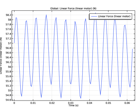
In the Settings window for Global, click Replace Expression in the upper-right corner of the y-Axis Data section. From the menu, choose Component 1 (comp1)>Definitions>Variables>Force - Linear Force (linear motor) - N.
3
In the Linear force toolbar, click  Plot.
Torque harmonics
1
In the Home toolbar, click  Add Plot Group and choose 1D Plot Group.
2
In the Settings window for 1D Plot Group, type Torque harmonics in the Label text field.
3
Locate the Data section. From the Dataset list, choose None.
Table Graph 1
1
Right-click Torque harmonics and choose Table Graph.
When performing the Fourier transform we will scale the x-axis in order to get the results as haromincs of the electrical frequency.
2
In the Settings window for Table Graph, locate the Data section.
3
From the x-axis data list, choose Time (s).
4
From the Plot columns list, choose Manual.
5
In the Columns list, select Torque (axial flux motor) (J).
6
From the Transformation list, choose Discrete Fourier transform.
7
From the Show list, choose Frequency spectrum.
8
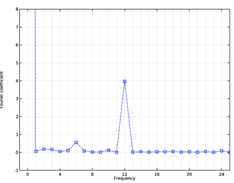
Click to expand the Preprocessing section. Find the x-axis column subsection. From the Preprocessing list, choose Linear.
9
In the Scaling text field, type f_el.
10
Locate the Coloring and Style section. Find the Line style subsection. From the Line list, choose Dashed.
11
Find the Line markers subsection. From the Marker list, choose Square.
12
From the Positioning list, choose In data points.
13
In the Torque harmonics toolbar, click  Plot.
Torque harmonics
1
In the Model Builder window, click Torque harmonics.
2
In the Settings window for 1D Plot Group, locate the Axis section.
3
Select the Manual axis limits check box.
4
In the x minimum text field, type -1.
5
In the x maximum text field, type 25.
6
In the y minimum text field, type -1.
7
In the y maximum text field, type 8.
8
Locate the Grid section. Select the Manual spacing check box.
9
In the Torque harmonics toolbar, click  Plot.