PDF

Inductive Heating of a Copper Cylinder
Introduction
The induced currents in a copper cylinder produce heat, and when the temperature rises, the electric conductivity of the copper changes. Solving the heat transfer simultaneously with the field propagation is therefore crucial for an accurate description of this process.
The heating caused by the induced currents is called inductive heating. Generally, heating due to currents is also called resistive heating or ohmic heating.
A challenge in induction heating is that the high current in the induction coils requires active cooling. This can be obtained by making the coil conductors hollow and circulating water inside. Even for rather modest flow rates, the coolant flow becomes highly turbulent which makes the heat transfer between conductor and fluid very efficient. This example illustrates a simplified way of modeling water cooling based on the assumption of turbulent flow and instantaneous mixing.
For mechanical support and electrical insulation, the cylinder and coil are embedded in FR4 composite material.
Model Definition
The system to be solved is given by
where ρ is the density, Cp is the specific heat capacity, k is the thermal conductivity, and Q is the inductive heating.
The electric conductivity of copper, σ, is given by the expression
where ρ0 is the resistivity at the reference temperature T0 = 293 K, α is the temperature coefficient of the resistivity, and T is the actual temperature in the domain.
The time average of the inductive heating over one period, is given by
The coil conductor is cooled by a turbulent water flow in an internal cooling channel. This is emulated by a combination of a high effective thermal conductivity and a homogenized out-of-plane convective loss term:
where is the water mass flow, Tin is the water inlet temperature, r is the radial coordinate and A is the cross-section area of the cooling channel.
Results and Discussion
The temperature after 10 h is shown in Figure 1. The average temperature of the copper cylinder has increased from 293 K to 346 K during this time. The current in the coil has an amplitude of 2 kA.
Figure 1: Temperature distribution after 10 h.
Figure 2: The plot shows the temperature evolution in the center of the copper cylinder and in the cooling channel.
Application Library path: ACDC_Module/Electromagnetic_Heating/inductive_heating
Modeling Instructions
From the File menu, choose New.
New
In the New window, click  Model Wizard.
Model Wizard
1
In the Model Wizard window, click  2D Axisymmetric.
2
In the Select Physics tree, select Heat Transfer>Electromagnetic Heating>Induction Heating.
3
Click Add.
4
Click  Study.
5
In the Select Study tree, select Preset Studies for Selected Multiphysics>Frequency-Transient.
6
Global Definitions
Parameters 1
1
In the Model Builder window, under Global Definitions click Parameters 1.
2
In the Settings window for Parameters, locate the Parameters section.
3
Geometry 1
Rectangle 1 (r1)
1
In the Geometry toolbar, click  Rectangle.
2
In the Settings window for Rectangle, locate the Size and Shape section.
3
In the Width text field, type 0.2.
4
In the Height text field, type 0.5.
5
Locate the Position section. In the z text field, type -0.25.
6
Click  Build Selected.
Rectangle 2 (r2)
1
In the Geometry toolbar, click  Rectangle.
2
In the Settings window for Rectangle, locate the Size and Shape section.
3
In the Width text field, type 0.03.
4
In the Height text field, type 0.1.
5
Locate the Position section. In the z text field, type -0.05.
6
Click  Build Selected.
Circle 1 (c1)
1
In the Geometry toolbar, click  Circle.
2
In the Settings window for Circle, locate the Size and Shape section.
3
In the Radius text field, type 0.01.
4
Locate the Position section. In the r text field, type 0.05.
5
Click  Build Selected.
Circle 2 (c2)
1
Right-click Circle 1 (c1) and choose Duplicate.
2
In the Settings window for Circle, locate the Size and Shape section.
3
In the Radius text field, type Rc.
4
Click  Build Selected.
Form Union (fin)
1
In the Model Builder window, click Form Union (fin).
2
In the Settings window for Form Union/Assembly, click  Build Selected.
Add Material
1
In the Home toolbar, click  Add Material to open the Add Material window.
2
Go to the Add Material window.
3
In the tree, select Built-in>FR4 (Circuit Board).
4
Click Add to Component in the window toolbar.
5
6
Click Add to Component in the window toolbar.
7
In the tree, select Built-in>Water, liquid.
8
Click Add to Component in the window toolbar.
9
In the Home toolbar, click  Add Material to close the Add Material window.
Materials
Copper (mat2)
1
In the Model Builder window, under Component 1 (comp1)>Materials click Copper (mat2).
2
3
In the Model Builder window, expand the Copper (mat2) node, then click Linearized resistivity (ltr).
4
In the Settings window for Linearized Resistivity, locate the Output Properties section.
5
Ω·m
Water, liquid (mat3)
1
In the Model Builder window, click Water, liquid (mat3).
2
The built-in water material does not provide the electric permittivity and the magnetic permeability. Add those values.
3
In the Settings window for Material, locate the Material Contents section.
4
Increase the thermal conductivity of the water to model the efficient heat transport in turbulent flow.
5
Magnetic Fields (mf)
Add a separate Ampère’s Law feature in the copper regions to specify a temperature-dependent resistivity.
Ampère’s Law 2
1
In the Model Builder window, under Component 1 (comp1) right-click Magnetic Fields (mf) and choose Ampère’s Law.
2
3
In the Settings window for Ampère’s Law, locate the Constitutive Relation Jc-E section.
4
From the Conduction model list, choose Linearized resistivity.
Coil 1
1
In the Physics toolbar, click  Domains and choose Coil.
2
3
In the Settings window for Coil, locate the Coil section.
4
In the Icoil text field, type I0.
Heat Transfer in Solids (ht)
Set up the Heat Transfer boundary conditions.
1
In the Model Builder window, under Component 1 (comp1) click Heat Transfer in Solids (ht).
Temperature 1
1
In the Physics toolbar, click  Boundaries and choose Temperature.
2
3
In the Settings window for Temperature, locate the Temperature section.
4
In the T0 text field, type T0.
Heat Source 1
1
In the Physics toolbar, click  Domains and choose Heat Source.
2
3
In the Settings window for Heat Source, locate the Heat Source section.
4
In the Q0 text field, type Mt*ht.Cp*(Tin-T)/(2*pi*r*Ac).
Mesh 1
In the Model Builder window, under Component 1 (comp1) right-click Mesh 1 and choose Build All.
Study 1
Step 1: Frequency-Transient
1
In the Model Builder window, under Study 1 click Step 1: Frequency-Transient.
2
In the Settings window for Frequency-Transient, locate the Study Settings section.
3
From the Time unit list, choose h.
4
Click  Range.
5
In the Range dialog box, type 10[min] in the Step text field.
6
In the Stop text field, type 10[h].
7
Click Replace.
8
In the Settings window for Frequency-Transient, locate the Study Settings section.
9
In the Frequency text field, type 500[Hz].
10
In the Home toolbar, click  Compute.
Results
Temperature, 3D (ht)
The revolution plot shows the temperature distribution after 10 hours; compare with Figure 1.
Create point datasets for plotting the temperature evolution in the copper cylinder and in the cooling channel.
Cut Point 2D 1
1
In the Model Builder window, expand the Results>Datasets node.
2
Right-click Results>Datasets and choose Cut Point 2D.
3
In the Settings window for Cut Point 2D, locate the Point Data section.
4
In the r text field, type 0.
5
In the z text field, type 0.
Cut Point 2D 2
1
Right-click Cut Point 2D 1 and choose Duplicate.
2
In the Settings window for Cut Point 2D, locate the Point Data section.
3
In the r text field, type 0.05.
1D Plot Group 5
In the Results toolbar, click  1D Plot Group.
Point Graph 1
1
Right-click 1D Plot Group 5 and choose Point Graph.
2
In the Settings window for Point Graph, locate the Data section.
3
From the Dataset list, choose Cut Point 2D 1.
4
From the Solution parameters list, choose From parent.
5
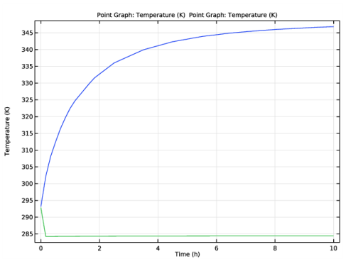
Click Replace Expression in the upper-right corner of the y-Axis Data section. From the menu, choose Component 1 (comp1)>Heat Transfer in Solids>Temperature>T - Temperature - K.
Point Graph 2
1
Right-click Point Graph 1 and choose Duplicate.
2
In the Settings window for Point Graph, locate the Data section.
3
From the Dataset list, choose Cut Point 2D 2.
4
In the 1D Plot Group 5 toolbar, click  Plot.
The plot shows the temperature evolution in the center of the copper cylinder and in the cooling channel; compare with Figure 2.
Finish the modeling session by saving a representative model thumbnail.
Temperature, 3D (ht)
Click the  Zoom Extents button in the Graphics toolbar.
Root
1
In the Model Builder window, click the root node.
2
In the root node’s Settings window, locate the Presentation section.
3
Find the Thumbnail subsection. Click Set from Graphics Window.