PDF

Force Calculation 3 — Magnetic Torque BEM FEM
Introduction
A common way to determine electromagnetic forces on a (rigid) body, is to integrate the stresses originating from jumps in the electromagnetic field on its exterior surface. These stresses can be expressed by means of the Maxwell surface stress tensor1. In case of magnetostatics, the surface stress tensor is based directly on the magnetic flux density B and the magnetic field H on the boundary. Therefore, an accurate force computation requires accurate knowledge of the boundary fluxes.
Within the context of the magnetic scalar potential formulation2, it makes sense to do a comparison between the boundary element method (BEM) and the finite element method (FEM). As opposed to the finite element method, for the boundary element method the flux normal to the boundary enters the equations directly as a degree of freedom. This allows for accurate flux computations without the need for reaction force integrals or weak constraints3. It is a potential advantage when doing force calculations.
In order to investigate the accuracy and general behavior of both methods, conditions are chosen for which the analytical solution is known. Results are analyzed. Mesh convergence is investigated by checking the behavior for different mesh sizes.
Model Definition
This model is a continuation of the Magnetic Force BEM FEM verification model. A single magnetized rod of one meter length, is placed in a perpendicular external field Be (see Figure 1). The relative permeability is assumed to be one everywhere. The strength of the external field is chosen such that the analytical model predicts a torque on the rod, of one newton-meter exactly.
The analytical model
In the Magnetic Force BEM FEM verification model (the previous tutorial in this series), the analogy between an electrostatics problem and the magnetic scalar potential formulation is used to establish an analytical model that describes the force between two magnetized rods. If you are new to this concept, consider starting with that tutorial first. In this tutorial, for the torque, a similar approach is chosen.
Figure 1: A single magnetized rod placed in a perpendicular external field. The situation is described analytically by means of two magnetic point charges forming a magnetic dipole.
A magnetized rod of one meter length, is described by means of two magnetic point charges qm1 and qm2 (in webers), at a distance of one meter apart (see Figure 1). The charge accumulated at the poles is the same as the one used for the two parallel rods discussed in the Magnetic Force BEM FEM model:
(1)
Again, in order to make the point charge approximation accurate the rod is given a thickness that is small compared to the other distances involved, making this rod identical to either one of the two rods discussed previously.
The two point charges form a magnetic dipole, having a magnetic dipole moment m (in ampere-meter2) equal to:
(2)
Here, l is a vector pointing from qm- to qm+, with a magnitude equal to the distance between the two charges (one meter in this case). The division by μ0 is essentially a unit conversion4 from the magnetic charge qm in webers, to the magnetic pole strength pm in ampere-meters. Now, for a given external field Be, the torque acting on this magnetic dipole is given by:
(3)
In a similar fashion, assuming the external field is oriented perpendicular with respect to the rod (that is, the angle θ is equal to 90°), we have:
(4)
Finally, given that m points in the negative x-direction, the external field needed in order to achieve one newton-meter of torque pointing in the positive y-direction, is given by:
(5)
This is all assuming the relative permeability equals one everywhere.
Modeling Approach
After setting up the general problem (geometry, physics, mesh, and such), two studies are performed. The first one focuses on the performance of the boundary element method alone. The second one repeats a similar investigation for a combined FEM-BEM model, where the finite element method is used to model the rod itself and its direct vicinity (marked as solid domains5, see Figure 2).
Both studies use the same geometry. The geometry contains a single rod enclosed by a force probe surface (for accurate torque calculation, see On Auxiliary Surfaces). The rod and the probe are contained in a solid sphere and a cubic surface. The cube is used for applying the external field. It is not depicted here, as it is about five times the size of the sphere.
Figure 2: A 2D representation of the used geometry. The solid parts are solved for using both FEM and BEM. The void is solved using the BEM only.
The mesh for the two studies is different. The first study uses a boundary mesh only, for the exterior surface of the rod, the force probe, and the cube. For the second study a volumetric mesh is added to the solid domains, as this is required for solving with the finite element method. Both studies use a parametric sweep to refine the mesh near the poles (see On Mesh Convergence Studies).
The results are investigated on the poles and on the force probe surface. Both for the BEM model as well as the combined FEM-BEM model, the total torque is determined as a function of the mesh refinement parameter.
On Auxiliary Surfaces
The total torque on the rod is determined by integrating the Maxwell surface stress tensor over its exterior boundaries, taking the torque axis into account. As the fields near the poles will be highly concentrated, so will the stress tensor. The quantity entering the boundary integral will therefore be concentrated in a few mesh elements only, with a value close to zero everywhere else. These conditions result in poor numerical accuracy.
If there is enough space around the body of interest, one alternative is to introduce an auxiliary surface enclosing it while keeping a certain distance (in this model, referred to as a force probe surface). Since the singular behavior that occurs near the poles fades away at a distance, the stress tensor behaves more nicely here. The resulting integral is much more accurate.
On Mesh Convergence Studies
A mesh convergence study typically refines the mesh in some region that is considered to be important. During postprocessing, the behavior of the result as a function of mesh refinement is analyzed. The general assumption is that a well-behaved model (one that does not contain singularities and such) will approach the “true” solution, as the mesh is further refined. Consequently, for any particular mesh, the mesh convergence study gives an indication as to the margin of error that may be expected.
You could interpret the mesh as the finite numerical resolution6 if you will, not to be confused with approximations done in the model itself. For example, the analytical model approximates the poles using point charges. This implies the rod is considered to be infinitely thin. As the actual rod used in the model has a finite thickness, the results will never perfectly correspond to the analytical model, even when using an infinitely fine mesh.
Results and Discussion
Mesh Convergence Study BEM
During the first study, an inspection of the Maxwell surface stress tensor on the rods poles shows that the boundary element method is capable of producing smooth fields, even for relatively coarse meshes (see Figure 3).
Figure 3: The Maxwell surface stress tensor at the rods pole, when using the boundary element method and a mesh scaling factor of one half.
Furthermore, the stresses are strongly concentrated on the fillets. This effect becomes more pronounced the smaller the radius of the fillet becomes. Without the fillet, the stress tensor would reach a singularity even. This is the reason why torque calculations on bodies with sharp edges are generally inaccurate7.
On the force probe surface, the results are more smooth (that is, less erratic and distributed over a larger surface area). The scale reaches a value of about 9.4 N/m2, as opposed to the value of ~5·104 N/m2 for the pole surface (see Figure 4).
Figure 4: The Maxwell surface stress tensor on the force probe surface.
When using the BEM and integrating over the rods exterior, one finds for the calculated total torque, an error of about ~0.02% to ~1% (depending on the mesh scaling parameter; see Figure 5). The torque calculated using the force probe surface is more constant, and settles around ~0.2%. These are decent figures for a numerical model like this, certainly when considering the analytical model isn’t a hundred percent accurate either.
Mesh Convergence Study FEM
During the second study, an inspection of the stress tensor on the rods poles shows singularities for low values of the mesh scaling factor hf. This is partly due to some of the mesh elements becoming linearized8. The linearized mesh elements are caused by the tetrahedra enclosing the curved surface (the tetrahedra are needed for solving with the FEM).
When comparing the total torque to the analytical model, an integration of the stress tensor over the rods surface gives an error that converges from somewhere in the interval 100–600% to about 0.3–7.0%, depending on hf. The force probe surface gives a more accurate value, at about 0.5–2.0%.
Figure 5: The error with respect to the analytical model, for both the rod surface integral and the probe surface integral, for both the BEM- and the combined FEM-BEM model.
Application Library path: ACDC_Module/Verification,_Forces/force_calculation_03_magnetic_torque_bem
Modeling Instructions
This first section discusses how to set up the geometry, the selections, the physics, and the mesh. The actual studies are performed in sections Modeling Instructions Mesh Convergence Study BEM, and Modeling Instructions Mesh Convergence Study FEM.
From the File menu, choose New.
New
In the New window, click  Model Wizard.
Model Wizard
1
In the Model Wizard window, click  3D.
2
In the Select Physics tree, select AC/DC>Magnetic Fields, No Currents>Magnetic Fields, No Currents, Boundary Elements (mfncbe).
3
Click Add.
4
In the Select Physics tree, select AC/DC>Magnetic Fields, No Currents>Magnetic Fields, No Currents (mfnc).
5
Click Add.
6
In the Select Physics tree, select AC/DC>Magnetic Fields, No Currents>Magnetic Fields, No Currents, Boundary Elements (mfncbe).
7
Click Add.
8
Click  Study.
9
In the Select Study tree, select General Studies>Stationary.
10
Geometry 1
As the main focus will be on the physics and numerics, a detailed treatment of the geometry building procedure lies outside the scope of this tutorial. Instead, the geometry has been prepared in the file force_calculation_01_introduction.mph. You can start by inserting the geometry sequence from that file.
1
In the Geometry toolbar, click  Insert Sequence.
2
3
In the Insert Sequence from File dialog box, select Geometry 2 (Magnetic Torque Verification) in the Select geometry sequence to insert list.
4
Form Union (fin)
1
In the Geometry toolbar, click  Build All.
2
Click the  Wireframe Rendering button in the Graphics toolbar.
3
Click the  Zoom Extents button in the Graphics toolbar.
You now have built the geometry. It contains a single rod in a spherical domain, encapsulated by a cubic surface. The sphere represents the boundary between the Magnetic Fields, No Currents interface, and the Magnetic Fields, No Currents, Boundary Elements 2 interface (see Figure 2). The cube will be used to apply the external field.
The modeling instructions for this geometry can be found in the Introduction tutorial (that is, the first model in this force verification series), section Modeling Instructions Magnetic Torque Verification Geometry.
If you have limited interest in manually building geometries in COMSOL Multiphysics (because you intend to use CAD software for example), feel free to proceed with setting the parameters and selections. If you are new to COMSOL however, it may be worthwhile to take some time and have a look at the instructions in the Introduction tutorial, as it will help you get familiar with the basics.
Global Definitions
Parameters 1
1
In the Model Builder window, under Global Definitions click Parameters 1.
2
In the Settings window for Parameters, locate the Parameters section.
Notice that the parameter list has been populated already. These five parameters (Rl, Ra, Rr, Rrf, and Cs) have been imported automatically, together with the geometry sequence that is based on them.
3
Click  Load from File.
4
Nine more items have been added to the list. The first two of these are related to the mesh and the geometry. The last seven represent the analytical model used to set the correct remanent flux density and external field strength. The parameters mu and Bez follow from Equation 2 and Equation 5 respectively.
In the following part, some selections are made. These selections will be used later on, when assigning domain features or building the mesh for instance.
In order to make life easier, you can define the selections by typing or pasting their list of entity numbers (as seen in the instructions for Explicit 3). If you want to practice using the selection tools in the Graphics window, you should try to reproduce the images and check whether the list of selected entities turns up the same (for details on selecting, panning and zooming, please consult the reference manual).
Definitions
Magnetized Rod Domain
1
In the Definitions toolbar, click  Explicit.
2
In the Settings window for Explicit, type Magnetized Rod Domain in the Label text field.
3
4
Click the  Zoom to Selection button in the Graphics toolbar.
Magnetized Rod Surface
1
In the Definitions toolbar, click  Adjacent.
2
In the Settings window for Adjacent, type Magnetized Rod Surface in the Label text field.
3
Locate the Input Entities section. Under Input selections, click  Add.
4
In the Add dialog box, select Magnetized Rod Domain in the Input selections list.
5
Magnetized Rod Pole Surface
1
In the Definitions toolbar, click  Explicit.
2
In the Settings window for Explicit, type Magnetized Rod Pole Surface in the Label text field.
3
Locate the Output Entities section. From the Output entities list, choose Adjacent boundaries.
4
5
Click the  Zoom to Selection button in the Graphics toolbar.
Magnetized Rod Pole Fillet
1
In the Definitions toolbar, click  Explicit.
2
In the Settings window for Explicit, type Magnetized Rod Pole Fillet in the Label text field.
3
Locate the Input Entities section. From the Geometric entity level list, choose Boundary.
4
Click  Paste Selection.
5
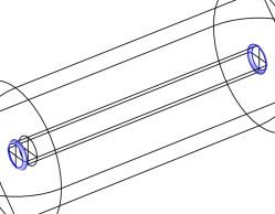
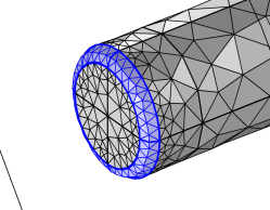
In the Paste Selection dialog box, type 17, 19, 22, 24, 42-45 in the Selection text field (that is, the boundaries comprising the pole fillets).
6
7
Click the  Zoom to Selection button in the Graphics toolbar.
Force Probe Domain
1
In the Definitions toolbar, click  Explicit.
2
In the Settings window for Explicit, type Force Probe Domain in the Label text field.
3
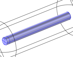
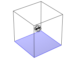
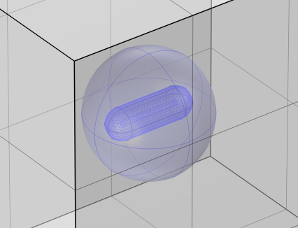
Select Domains 2–4 only (that is, both the magnetized rod, as well as the domain enclosing it).
4
Click the  Zoom to Selection button in the Graphics toolbar.
Force Probe Surface
1
In the Definitions toolbar, click  Adjacent.
2
In the Settings window for Adjacent, type Force Probe Surface in the Label text field.
3
Locate the Input Entities section. Under Input selections, click  Add.
4
In the Add dialog box, select Force Probe Domain in the Input selections list.
5
External Field In
1
In the Definitions toolbar, click  Explicit.
2
In the Settings window for Explicit, type External Field In in the Label text field.
3
Click the  Zoom Extents button in the Graphics toolbar.
4
Locate the Input Entities section. From the Geometric entity level list, choose Boundary.
5
External Field Out
1
In the Definitions toolbar, click  Explicit.
2
In the Settings window for Explicit, type External Field Out in the Label text field.
3
Locate the Input Entities section. From the Geometric entity level list, choose Boundary.
4
Exterior Cube Surface
1
In the Definitions toolbar, click  Explicit.
2
In the Settings window for Explicit, type Exterior Cube Surface in the Label text field.
3
Locate the Input Entities section. From the Geometric entity level list, choose Boundary.
4
Click  Paste Selection.
5
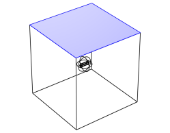
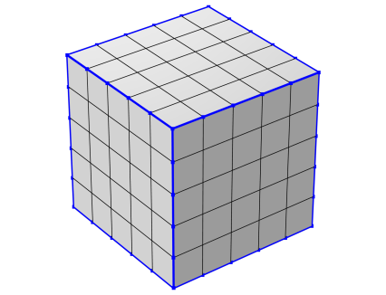
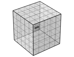
In the Paste Selection dialog box, type 1-5, 54 in the Selection text field (that is, the boundaries comprising the cube).
6
Materials
Next, will be the materials. For this model we only have one material, with a relative permeability of one everywhere. Please make sure the material selection is set to All domains and voids. Here, a “void” represents a domain that will not be meshed. Still, the boundary element method is able to solve for it. This is one of the main advantages of the BEM, when compared to the finite element method (for more information on this, please consult the reference manual).
Material 1 (mat1)
1
In the Model Builder window, under Component 1 (comp1) right-click Materials and choose Blank Material.
2
In the Settings window for Material, locate the Geometric Entity Selection section.
3
From the Selection list, choose All domains and voids.
4
Locate the Material Contents section. In the table, enter the following settings:
Magnetic Fields, No Currents, Boundary Elements (mfncbe)
Now that the materials have been set and double-checked, let us have a look at the physics. The first physics interface, Magnetic Fields, No Currents, Boundary Elements, is used for solving the entire model using the boundary element method only. The second and third interface will be coupled. Magnetic Fields, No Currents will solve a finite element problem in the rod itself and its direct vicinity (see Figure 2). Magnetic Fields, No Currents, Boundary Elements 2 will solve a boundary element problem for the cubic void only.
Start with the first physics interface, by setting the correct selection and adjusting the far-field approximation tolerance.
1
In the Model Builder window, under Component 1 (comp1) click Magnetic Fields, No Currents, Boundary Elements (mfncbe).
2
In the Settings window for Magnetic Fields, No Currents, Boundary Elements, locate the Domain Selection section.
3
Click  Clear Selection.
4
Click  Paste Selection.
5
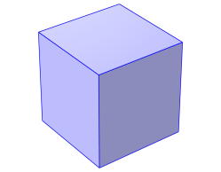
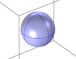
In the Paste Selection dialog box, type -1, 1-4 in the Selection text field (that is, everything except the infinite void). Notice that finite voids are indicated with a negative domain number. The infinite void is numbered 0.
6
7
Click the  Show More Options button in the Model Builder toolbar.
8
In the Show More Options dialog box, in the tree, select the check box for the node Physics>Advanced Physics Options.
9
10
In the Settings window for Magnetic Fields, No Currents, Boundary Elements, click to expand the Far-Field Approximation section.
11
In the Relative tolerance text field, type 1e-6.
Reducing the relative tolerance for the far-field approximation improves the accuracy of the BEM solution, without hindering performance too much (for more information on the far-field approximation settings, please consult the reference manual or use context help).
Next, add separate flux conservation features for the force probe domain and the magnetized rod. This will allow for determining the Maxwell surface stress tensor on their exterior boundaries.
Magnetic Flux Conservation 2
1
In the Physics toolbar, click  Domains and choose Magnetic Flux Conservation.
2
In the Settings window for Magnetic Flux Conservation, locate the Domain Selection section.
3
From the Selection list, choose Force Probe Domain.
4
Click the  Zoom to Selection button in the Graphics toolbar.
Magnetic Flux Conservation 3
1
In the Physics toolbar, click  Domains and choose Magnetic Flux Conservation.
2
In the Settings window for Magnetic Flux Conservation, locate the Domain Selection section.
3
From the Selection list, choose Magnetized Rod Domain.
4
Locate the Constitutive Relation B-H section. From the Magnetization model list, choose Remanent flux density.
5
From the  ||  Br   ||  list, choose User defined. In the associated text field, type sqrt(Brx^2+Brz^2).
6
Specify the e vector as
Observe that the second magnetic flux conservation feature partly overrides the first one. Therefore, it is important to have them in this order: the probe domain first, the rod domain second. For the force calculation features the order is less important.
Force Calculation 1
1
In the Physics toolbar, click  Domains and choose Force Calculation.
2
In the Settings window for Force Calculation, locate the Domain Selection section.
3
From the Selection list, choose Magnetized Rod Domain.
4
Locate the Force Calculation section. In the Force name text field, type BEM_rod.
5
Specify the rax vector as
Force Calculation 2
1
In the Physics toolbar, click  Domains and choose Force Calculation.
2
In the Settings window for Force Calculation, locate the Domain Selection section.
3
From the Selection list, choose Force Probe Domain.
4
Locate the Force Calculation section. In the Force name text field, type BEM_probe.
5
Specify the rax vector as
These force calculation features provide the machinery for automated torque calculation. The total torque on the chosen domain selection will be determined by integrating the stress tensor over its exterior boundaries, taking the torque axis into account.
Finally, apply the external field. In order to see the selections for the exterior boundary conditions, zoom out a bit.
6
Click the  Zoom Extents button in the Graphics toolbar.
Magnetic Flux Density 1
1
In the Physics toolbar, click  Boundaries and choose Magnetic Flux Density.
2
In the Settings window for Magnetic Flux Density, locate the Boundary Selection section.
3
From the Selection list, choose External Field In.
4
Locate the Magnetic Flux Density section. In the Bn text field, type Bez.
Zero Magnetic Scalar Potential 1
1
In the Physics toolbar, click  Boundaries and choose Zero Magnetic Scalar Potential.
2
In the Settings window for Zero Magnetic Scalar Potential, locate the Boundary Selection section.
3
From the Selection list, choose External Field Out.
Notice that the zero scalar potential boundary condition actually serves a double purpose. First of all, it is an equipotential surface forcing the field in a vertical direction near the boundary. Secondly, it provides a zero potential reference, making the scalar potential field unique. Without it, only its spatial derivative would be unique and solving with a direct solver would not work (for details on under constrained problems, please consult the reference manual).
The next two interfaces will essentially perform the same simulation as the first one. Observe that the Magnetic Fields, No Currents interface does not need a zero potential constraint (since it will be coupled).
What remains are the settings for the remanent flux density and the force calculation features. Proceed by adding them.
Magnetic Fields, No Currents (mfnc)
1
Click the  Zoom to Selection button in the Graphics toolbar.
2
In the Model Builder window, under Component 1 (comp1) click Magnetic Fields, No Currents (mfnc).
Magnetic Flux Conservation 2
1
In the Physics toolbar, click  Domains and choose Magnetic Flux Conservation.
2
In the Settings window for Magnetic Flux Conservation, locate the Domain Selection section.
3
From the Selection list, choose Magnetized Rod Domain.
4
Locate the Constitutive Relation B-H section. From the Magnetization model list, choose Remanent flux density.
5
From the  ||  Br   ||  list, choose User defined. In the associated text field, type sqrt(Brx^2+Brz^2).
6
Specify the e vector as
Notice that the finite element method does not need a separate flux conservation feature for the probe domain. This is because for the FEM, all boundaries within the physics domain selection will be equipped with the appropriate boundary variable definitions by default (the surface stress tensor in this case). The BEM on the other hand, only defines these variables for the boundaries that it solves for.
Force Calculation 1
1
In the Physics toolbar, click  Domains and choose Force Calculation.
2
In the Settings window for Force Calculation, locate the Domain Selection section.
3
From the Selection list, choose Magnetized Rod Domain.
4
Locate the Force Calculation section. In the Force name text field, type FEM_rod.
5
Specify the rax vector as
Force Calculation 2
1
In the Physics toolbar, click  Domains and choose Force Calculation.
2
In the Settings window for Force Calculation, locate the Domain Selection section.
3
From the Selection list, choose Force Probe Domain.
4
Locate the Force Calculation section. In the Force name text field, type FEM_probe.
5
Specify the rax vector as
6
Click the  Zoom Extents button in the Graphics toolbar.
Magnetic Fields, No Currents, Boundary Elements 2 (mfncbe2)
The last interface solves for the void between the sphere and the cube. It applies the same exterior boundary conditions as the Magnetic Fields, No Currents, Boundary Elements interface.
1
In the Model Builder window, under Component 1 (comp1) click Magnetic Fields, No Currents, Boundary Elements 2 (mfncbe2).
2
In the Settings window for Magnetic Fields, No Currents, Boundary Elements, locate the Domain Selection section.
3
Click  Clear Selection.
4
Click  Paste Selection.
5
In the Paste Selection dialog box, type -1 in the Selection text field (that is, just the finite void).
6
Magnetic Flux Density 1
1
In the Physics toolbar, click  Boundaries and choose Magnetic Flux Density.
2
In the Settings window for Magnetic Flux Density, locate the Boundary Selection section.
3
From the Selection list, choose External Field In.
4
Locate the Magnetic Flux Density section. In the Bn text field, type Bez.
Zero Magnetic Scalar Potential 1
1
In the Physics toolbar, click  Boundaries and choose Zero Magnetic Scalar Potential.
2
In the Settings window for Zero Magnetic Scalar Potential, locate the Boundary Selection section.
3
From the Selection list, choose External Field Out.
If this selection shows up as “non applicable”, it probably means for the physics interface you have selected one void too much (it should only be “Finite void 1”).
Multiphysics
Magnetic Scalar-Scalar Potential Coupling 1 (msspc1)
1
In the Physics toolbar, click  Multiphysics Couplings and choose Boundary>Magnetic Scalar-Scalar Potential Coupling.
2
In the Settings window for Magnetic Scalar-Scalar Potential Coupling, locate the Coupled Interfaces section.
3
From the Secondary interface (magnetic scalar potential) list, choose Magnetic Fields, No Currents, Boundary Elements 2 (mfncbe2).
4
Locate the Boundary Selection section. From the Selection list, choose All boundaries.
5
Click the  Zoom to Selection button in the Graphics toolbar.
This coupling constrains the difference between the FEM scalar potential and the BEM scalar potential to zero on the boundary (that is, it makes them equal).
Mesh 1
Next will be a manual mesh. Special care is taken to create a fine mesh for the fillets on the magnetized rod.
1
In the Model Builder window, under Component 1 (comp1) click Mesh 1.
2
In the Settings window for Mesh, locate the Physics-Controlled Mesh section.
3
From the Element size list, choose Finer.
Free Triangular 1
1
In the Mesh toolbar, click  Boundary and choose Free Triangular.
2
In the Settings window for Free Triangular, locate the Boundary Selection section.
3
From the Selection list, choose Magnetized Rod Surface.
Size 1
1
Right-click Free Triangular 1 and choose Size.
2
In the Settings window for Size, locate the Geometric Entity Selection section.
3
From the Selection list, choose Magnetized Rod Pole Fillet.
4
Locate the Element Size section. Click the Custom button.
5
Locate the Element Size Parameters section. Select the Maximum element size check box.
6
7
Click  Build All.
Notice that the mesh uses the parameter hf. Setting this parameter from 1 to 2 and so on, refines the mesh on the fillet. This will be of particular interest during the mesh convergence studies.
Free Triangular 2
1
In the Mesh toolbar, click  Boundary and choose Free Triangular.
2
In the Settings window for Free Triangular, locate the Boundary Selection section.
3
From the Selection list, choose Force Probe Surface.
Size 1
1
Right-click Free Triangular 2 and choose Size.
2
In the Settings window for Size, locate the Element Size section.
3
Click the Custom button.
4
Locate the Element Size Parameters section. Select the Maximum element size check box.
5
6
Click  Build All.
7
Click the  Zoom to Selection button in the Graphics toolbar.
As the force probe surface mesh does not depend on the parameter hf, it will not vary during the mesh convergence study.
Mapped 1
1
In the Mesh toolbar, click  Boundary and choose Mapped.
2
In the Settings window for Mapped, locate the Boundary Selection section.
3
From the Selection list, choose Exterior Cube Surface.
Distribution 1
1
Right-click Mapped 1 and choose Distribution.
2
In the Settings window for Distribution, locate the Edge Selection section.
3
From the Selection list, choose All edges.
4
Click  Build All.
5
Click the  Zoom to Selection button in the Graphics toolbar.
Modeling Instructions — Mesh Convergence Study BEM
Study 1
A mesh convergence study typically investigates the behavior of the result as a function of mesh refinement (see section On Mesh Convergence Studies). For any particular mesh, the mesh convergence study gives an indication as to the margin of error that may be expected.
1
In the Model Builder window, click Study 1.
2
In the Settings window for Study, locate the Study Settings section.
3
Clear the Generate default plots check box.
Parametric Sweep
1
In the Study toolbar, click  Parametric Sweep.
2
In the Settings window for Parametric Sweep, locate the Study Settings section.
3
4
In the table, enter the following settings (make sure the parameter unit is cleared):
Step 1: Stationary
1
In the Model Builder window, click Step 1: Stationary.
2
In the Settings window for Stationary, locate the Physics and Variables Selection section.
3
Before hitting compute, it is recommended to save your model.
Solving should take about 5 minutes on an average desktop machine. The required RAM is somewhere around 6 GB. If the model is too demanding for your current setup, consider changing the parameter setting hf from 0.5 1 2, to 0.5 1 (that is, solving for the coarser meshes only).
4
In the Study toolbar, click  Compute.
Results
Since the main region of interest lies inside the sphere, it is convenient to add a selection to the solution (All domains in this case). This will force the plots to exclude the cube (which is a void).
In the Model Builder window, expand the Results node.
Study 1/Solution 1 (sol1)
In the Model Builder window, expand the Results>Datasets node, then click Study 1/Solution 1 (sol1).
Selection
1
In the Results toolbar, click  Attributes and choose Selection.
2
In the Settings window for Selection, locate the Geometric Entity Selection section.
3
From the Geometric entity level list, choose Domain.
4
From the Selection list, choose All domains.
5
Click the  Zoom to Selection button in the Graphics toolbar.
The first plot group considers the norm of the surface stress tensor on the poles. The stress tensor plot will be combined with a mesh plot, to show the relation between the mesh and the resulting fields. Start by adding a new plot group.
Maxwell Surface Stress Tensor (BEM Rod)
1
In the Results toolbar, click  3D Plot Group.
2
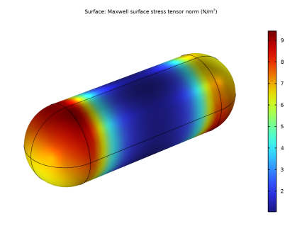
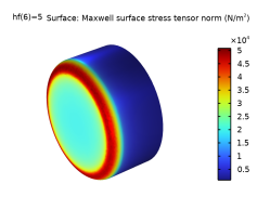
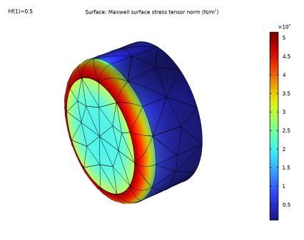
In the Settings window for 3D Plot Group, type Maxwell Surface Stress Tensor (BEM Rod) in the Label text field.
3
Locate the Data section. From the Dataset list, choose Study 1/Parametric Solutions 1 (sol2).
4
From the Parameter value (hf) list, choose 0.5.
5
Locate the Plot Settings section. Clear the Plot dataset edges check box.
6
Click to expand the Selection section. From the Geometric entity level list, choose Boundary.
7
From the Selection list, choose Magnetized Rod Pole Surface.
Surface 1
1
Right-click Maxwell Surface Stress Tensor (BEM Rod) and choose Surface.
2
In the Settings window for Surface, locate the Expression section.
3
In the Expression text field, type sqrt(mfncbe.nTx_BEM_rod^2+mfncbe.nTy_BEM_rod^2+mfncbe.nTz_BEM_rod^2).
Notice that for longer expressions like this one, the easiest way to go, is to copy-paste them directly from this *.pdf file to COMSOL.
Variables like mfncbe.nTx_BEM_rod have been generated by the force calculation features. You can find them using the buttons in the top-right corner of the Expression section, just above the text input field for the expression. There is some autocomplete functionality too (try hitting Ctrl+Space, when having focus in the text input field).
4
Select the Description check box.
5
In the associated text field, type Maxwell surface stress tensor norm.
6
In the Maxwell Surface Stress Tensor (BEM Rod) toolbar, click  Plot.
7
Click the  Zoom Extents button in the Graphics toolbar.
Surface 2
1
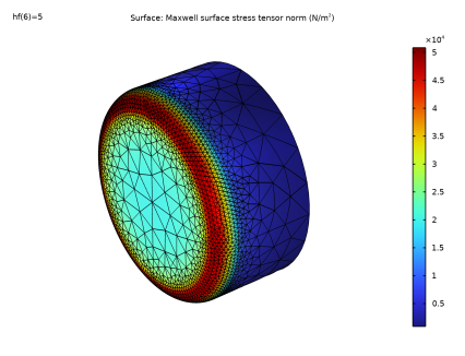
In the Model Builder window, right-click Maxwell Surface Stress Tensor (BEM Rod) and choose Surface.
2
In the Settings window for Surface, locate the Expression section.
3
In the Expression text field, type 0.
4
Click to expand the Title section. From the Title type list, choose None.
5
Locate the Coloring and Style section. From the Coloring list, choose Uniform.
6
From the Color list, choose Black.
7
Select the Wireframe check box.
8
In the Maxwell Surface Stress Tensor (BEM Rod) toolbar, click  Plot.
One of the things to notice, is that the solution depends on the chosen mesh. Feel free to investigate the plot for different values of the mesh scaling factor hf.
Next, create a plot for the surface stress tensor on the force probe surface.
Maxwell Surface Stress Tensor (BEM Probe)
1
In the Home toolbar, click  Add Plot Group and choose 3D Plot Group.
2
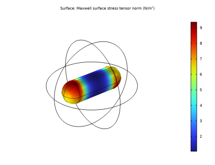
In the Settings window for 3D Plot Group, type Maxwell Surface Stress Tensor (BEM Probe) in the Label text field.
Since the probe surface is much larger than the rod pole, it is convenient to have two separate views. This way, the first view can be kept zoomed in on the pole, while the second one focuses on the probe. Using a single view for both, would result in having to adjust the camera settings, every time when switching between the first and second plot group.
3
Locate the Plot Settings section. From the View list, choose New view.
Surface 1
1
Right-click Maxwell Surface Stress Tensor (BEM Probe) and choose Surface.
2
In the Settings window for Surface, locate the Expression section.
3
In the Expression text field, type sqrt(mfncbe.nTx_BEM_probe^2+mfncbe.nTy_BEM_probe^2+mfncbe.nTz_BEM_probe^2).
4
Select the Description check box.
5
In the associated text field, type Maxwell surface stress tensor norm.
6
In the Maxwell Surface Stress Tensor (BEM Probe) toolbar, click  Plot.
7
Click the  Zoom Extents button in the Graphics toolbar.
The field is more smooth here. The scale reaches a value of about 9.4 N/m2, as opposed to the value of ~5·104 N/m2 for the pole surface.
Finally, evaluate the error for the total torque as a function of hf. The error norm  ||δ||  is expressed in terms of the norm of the difference between the calculated torque vector T and the analytical result τ, that is:  ||δ|| = ((Tx −τ x)2 + (Ty −τ y)2 + (Tz −τ z)2)1/2.
In this case, for the analytical result we have τ = [0,1,0]T. Notice that since the analytical result has a magnitude of one, the error can be interpreted both as a relative (dimensionless) error, or as an absolute error (in Newton-meters).
Global Evaluation 1
1
In the Results toolbar, click  Global Evaluation.
2
In the Settings window for Global Evaluation, locate the Data section.
3
From the Dataset list, choose Study 1/Parametric Solutions 1 (sol2).
4
Locate the Expressions section. In the table, enter the following settings:
5
Click  Evaluate.
Table
1
Go to the Table window.
For the BEM rod, the error should be about ~0.02% to ~1%, depending on hf. The BEM probe result is more constant, and settles around ~0.2%.
Modeling Instructions — Mesh Convergence Study FEM
Mesh 1
For this part, the finite element interface Magnetic Fields, No Currents is used. Therefore, some domains will have to be meshed using a tetrahedral mesh (indicated with “solid” in Figure 2). Start by creating a duplicate of the BEM mesh.
In the Model Builder window, under Component 1 (comp1) right-click Mesh 1 and choose Duplicate.
Mesh 2
1
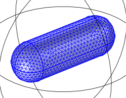
In the Model Builder window, under Component 1 (comp1)>Meshes right-click Mesh 2 and choose Build All.
2
Click the  Zoom Extents button in the Graphics toolbar.
3
Click the  Transparency button in the Graphics toolbar.
Free Tetrahedral 1
1
In the Mesh toolbar, click  Free Tetrahedral.
2
In the Settings window for Free Tetrahedral, click  Build All.
3
Click the  Zoom to Selection button in the Graphics toolbar.
Notice that only the sphere has been filled with tetrahedra, not the cube. This is because the sphere is a solid domain, whereas the cube is a surface (a void). The setting responsible for this is the cube’s Object Type.
4
Click the  Transparency button in the Graphics toolbar.
5
Click the  Zoom Extents button in the Graphics toolbar.
Next, add a new study, specifically for the two coupled physics interfaces.
Add Study
1
In the Home toolbar, click  Add Study to open the Add Study window.
2
Go to the Add Study window.
3
Find the Physics interfaces in study and Multiphysics couplings in study subsections. In the tables, enter the following settings:
4
Find the Studies subsection. In the Select Study tree, select General Studies>Stationary.
5
6
In the Home toolbar, click  Add Study to close the Add Study window.
Study 2
1
In the Settings window for Study, locate the Study Settings section.
2
Clear the Generate default plots check box.
Parametric Sweep
1
In the Study toolbar, click  Parametric Sweep.
2
In the Settings window for Parametric Sweep, locate the Study Settings section.
3
4
In the table, enter the following settings (make sure the parameter unit is cleared):
Step 1: Stationary
Before hitting compute, it is recommended to save your model.
Solving should take about 4 minutes on an average desktop machine. The required RAM is somewhere around 6 GB. If the model is too demanding for your current setup, consider changing the parameter setting hf from 0.5 1 2 3 4 5, to 0.5 1 2 3 (that is, solving for the coarser meshes only).
1
In the Study toolbar, click  Compute.
Results
First, add a selection to the solution (All domains, in the same fashion as done for the BEM study).
Study 2/Solution 6 (sol6)
In the Model Builder window, under Results>Datasets click Study 2/Solution 6 (sol6).
Selection
1
In the Results toolbar, click  Attributes and choose Selection.
2
In the Settings window for Selection, locate the Geometric Entity Selection section.
3
From the Geometric entity level list, choose Domain.
4
From the Selection list, choose All domains.
5
Click the  Zoom to Selection button in the Graphics toolbar.
The next plot group will be about the norm of the surface stress tensor on the poles (as for the BEM study).
Maxwell Surface Stress Tensor (FEM Rod)
1
In the Results toolbar, click  3D Plot Group.
2
In the Settings window for 3D Plot Group, type Maxwell Surface Stress Tensor (FEM Rod) in the Label text field.
3
Locate the Data section. From the Dataset list, choose Study 2/Parametric Solutions 2 (sol7).
4
Locate the Plot Settings section. Clear the Plot dataset edges check box.
5
Locate the Selection section. From the Geometric entity level list, choose Boundary.
6
From the Selection list, choose Magnetized Rod Pole Surface.
Surface 1
1
Right-click Maxwell Surface Stress Tensor (FEM Rod) and choose Surface.
2
In the Settings window for Surface, locate the Expression section.
3
In the Expression text field, type sqrt(mfnc.nTx_FEM_rod^2+mfnc.nTy_FEM_rod^2+mfnc.nTz_FEM_rod^2).
4
Select the Description check box.
5
In the associated text field, type Maxwell surface stress tensor norm.
6
In the Maxwell Surface Stress Tensor (FEM Rod) toolbar, click  Plot.
7
Click the  Zoom Extents button in the Graphics toolbar.
Surface 2
1
In the Model Builder window, right-click Maxwell Surface Stress Tensor (FEM Rod) and choose Surface.
2
In the Settings window for Surface, locate the Expression section.
3
In the Expression text field, type 0.
4
Locate the Title section. From the Title type list, choose None.
5
Locate the Coloring and Style section. From the Coloring list, choose Uniform.
6
From the Color list, choose Black.
7
Select the Wireframe check box.
8
In the Maxwell Surface Stress Tensor (FEM Rod) toolbar, click  Plot.
Again, feel free to investigate the plot for different values of the mesh scaling factor hf.
Next, create a plot for the surface stress tensor on the force probe surface.
Maxwell Surface Stress Tensor (FEM Probe)
1
In the Home toolbar, click  Add Plot Group and choose 3D Plot Group.
2
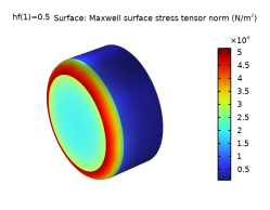
In the Settings window for 3D Plot Group, type Maxwell Surface Stress Tensor (FEM Probe) in the Label text field.
3
Locate the Data section. From the Dataset list, choose Study 2/Solution 6 (sol6).
Select a suitable view (notice that this view has been created when selecting a new view for the second plot group).
4
Locate the Plot Settings section. From the View list, choose View 3D 3.
Surface 1
1
Right-click Maxwell Surface Stress Tensor (FEM Probe) and choose Surface.
2
In the Settings window for Surface, locate the Expression section.
3
In the Expression text field, type sqrt(mfnc.nTx_FEM_probe^2+mfnc.nTy_FEM_probe^2+mfnc.nTz_FEM_probe^2).
4
Select the Description check box.
5
In the associated text field, type Maxwell surface stress tensor norm.
6
In the Maxwell Surface Stress Tensor (FEM Probe) toolbar, click  Plot.
7
Click the  Zoom Extents button in the Graphics toolbar.
Notice that just as for the BEM study, the field is more smooth here.
Evaluate the error for the total torque as a function of hf. Since the analytical result has a magnitude of one, the error can be interpreted both as a relative (dimensionless) error, or as an absolute error (in Newton-meters).
Global Evaluation 2
1
In the Results toolbar, click  Global Evaluation.
2
In the Settings window for Global Evaluation, locate the Data section.
3
From the Dataset list, choose Study 2/Parametric Solutions 2 (sol7).
4
Locate the Expressions section. In the table, enter the following settings:
5
Click  Evaluate.
Table
1
Go to the Table window.
For the FEM rod, the error should converge from somewhere in the interval 100–600% to about 0.3–7.0%, depending on hf. The FEM probe result is generally more accurate, at about 0.5–2.0%.
Results
Finally, create a table graph in order to show these results in a more comprehensible form.
Magnetic Torque Error
1
In the Results toolbar, click  1D Plot Group.
2
In the Settings window for 1D Plot Group, type Magnetic Torque Error in the Label text field.
3
Click to expand the Title section. From the Title type list, choose Manual.
4
In the Title text area, type Mesh convergence of magnetic torque.
5
Locate the Plot Settings section. Select the x-axis label check box.
6
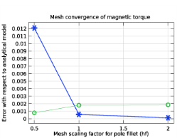
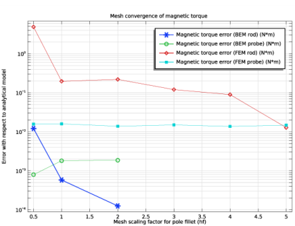
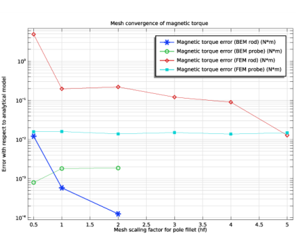
In the associated text field, type Mesh scaling factor for pole fillet (hf).
7
Select the y-axis label check box.
8
In the associated text field, type Error with respect to analytical model.
Table Graph 1
1
Right-click Magnetic Torque Error and choose Table Graph.
2
In the Settings window for Table Graph, locate the Coloring and Style section.
3
Find the Line markers subsection. From the Marker list, choose Cycle.
4
From the Positioning list, choose In data points.
5
Click to expand the Legends section. Select the Show legends check box.
6
In the Magnetic Torque Error toolbar, click  Plot.
Table Graph 2
1
In the Model Builder window, right-click Magnetic Torque Error and choose Table Graph.
2
In the Settings window for Table Graph, locate the Data section.
3
From the Table list, choose Table 2.
4
Locate the Coloring and Style section. Find the Line markers subsection. From the Marker list, choose Cycle.
5
From the Positioning list, choose In data points.
6
Locate the Legends section. Select the Show legends check box.
7
In the Magnetic Torque Error toolbar, click  Plot.
8
Click the  y-Axis Log Scale button in the Graphics toolbar.
Observe that the log scale is a very effective tool for displaying convergence behavior. Without it, only the “FEM rod” curve would be clearly distinguishable from the others.
In conclusion, these results show great potential for the boundary element method, even though its implementation in COMSOL Multiphysics is fairly new.
You have now completed this tutorial series, the other tutorials in this series will refer to the resulting file as force_calculation_03_magnetic_torque_bem.mph.
 

1
For more information about the Maxwell surface stress tensor, see the chapter on Electromagnetic Forces in the AC/DC Module User’s Guide.

2
This is the formulation used by the Magnetic Fields, No Currents and the Magnetic Fields, No Currents, Boundary Elements interfaces. For more information on this formulation, see the AC/DC Module User’s Guide.

3
For more information on flux computation methods, see the chapter Computing Accurate Fluxes in the COMSOL Multiphysics Reference Manual.

4
Notice that in SI units, there are two conflicting units in use for magnetic charge: webers and ampere-meters.

5
Here, “solid” refers to a geometrical entity that can be equipped with a volumetric mesh. Objects of type “surface” on the other hand, can only be equipped by a boundary mesh. Their interior is referred to as a void.

6
That is, taking the shape functions into account.

7
Notice that this specifically applies to methods based on surface integration; volume integration may be a different matter.

8
If a shape shows strong curvature with respect to the mesh element size, a second-order mesh element may become inverted. That is, its boundaries may become self-overlapping. Usually, as a fallback, linear mesh elements are chosen. For more information on inverted mesh elements, see the COMSOL Multiphysics Reference Manual.